🧲 Dynamic simulations

Power systems do not live still. They swing, accelerate, saturate, switch, ring, recover, and sometimes misbehave spectacularly. That is why VeraGrid has dynamic simulations.

Dynamic simulations are used to study the time evolution of electrical systems after disturbances, set-point changes, switching actions, or control responses. In VeraGrid, dynamic simulations are available in two main domains:

Root Mean Square (RMS): phasor-domain dynamic simulation for electromechanical and controller time scales.
Electromagnetic Transients (EMT): electromagnetic-transient simulation for waveform-level and switching-level phenomena.

Dynamic simulation is one of the main differences between a grid analysis platform that only solves steady-state operating points and one that can represent the actual temporal behavior of the system. For steady-state studies, the network is assumed to be already in equilibrium. For dynamic studies, the transient path between equilibria, or the possible loss of equilibrium, is the object of interest.

If power flow tells you where the system is standing, dynamic simulation tells you what happens when you poke it.

The classical theoretical foundations for power-system dynamic simulation can be found in Kundur’s treatment of electromechanical stability, in Milano’s differential-algebraic modelling framework, and in standard EMT references such as Dommel and Mahseredjian’s ATP/EMTP-oriented literature and the EMTP-RV theory texts [1]-[6]. VeraGrid follows the same general modelling philosophy: represent the network and devices as coupled differential-algebraic systems, initialize them consistently from a solved operating point, and integrate them in time with suitable numerical methods.

Why dynamic simulations are different from static simulations

Static simulations such as power flow, short circuit, or linearized analyses answer questions about one operating point or one algebraic condition. Dynamic simulations answer questions about the trajectory that follows a disturbance.

Typical dynamic questions are:

Does the system remain synchronized after a load step or a fault?
How does frequency evolve after a generation imbalance?
How do converter controls react to a voltage sag?
What is the bus-voltage waveform during a switching transient?
How do currents, internal states, and control references evolve in time?

For this reason, dynamic simulations require additional ingredients that static simulations do not:

Dynamic device models.
Initial values for states and algebraic variables.
Time-domain events.
Numerical integration methods.
Post-processing of trajectories instead of single operating-point values.

In VeraGrid, this means that a dynamic study is usually built on top of a static grid model, normally after a power-flow solution has been obtained.

RMS and EMT

VeraGrid supports two complementary dynamic simulation domains.

In the literature, dynamic power-system simulations are commonly grouped according to how electrical quantities are represented and which time scales are retained [1]-[5]. Two broad families dominate practical engineering work:

phasor or RMS-domain simulations, which focus on the slower electromechanical and control dynamics,
electromagnetic transient (EMT) simulations, which focus on instantaneous waveform dynamics.

The difference is not only numerical. It is also conceptual. Each domain is based on a different approximation of the same physical network.

RMS

RMS means root-mean-square phasor-domain simulation. The network variables are represented by slowly varying fundamental-frequency quantities instead of instantaneous phase waveforms. RMS simulation is appropriate when the electromagnetic transients inside one cycle are not the main object of study, but electromechanical dynamics, converter outer-loop controls, or slower controller interactions are.

In RMS simulation, voltages and currents are usually represented by phasor quantities or by state-space variables referred to one synchronous frame. The rapid oscillation at the fundamental frequency is not integrated explicitly in the same way as in EMT. Instead, the model tracks the evolution of slowly varying electrical and control quantities. This makes RMS simulation extremely valuable for system-wide transient stability studies [1]-[4].

From a modelling viewpoint, RMS simulation relies on the idea that many fast network transients can be neglected when the objective is to study slower system phenomena. The network is then represented by algebraic constraints, while the slow device dynamics are retained explicitly. A large part of classical transient-stability theory is based on this approximation.

Typical RMS applications are:

Rotor-angle and frequency stability.
AVR, governor, PSS, and plant-control studies.
Converter control studies where switching is not explicitly modelled.
Small disturbances, set-point changes, and medium-speed events.
Large multi-machine systems where computational efficiency matters.

The modelling philosophy is aligned with standard transient-stability formulations described by Kundur and Milano [1]-[3].

Typical RMS formulations in practice include:

balanced positive-sequence models,
unbalanced phasor-domain extensions,
dq-based averaged converter models,
phasor-domain machine and controller models.

In the context of VeraGrid, the currently consolidated RMS workflow is the balanced phasor-domain dynamic-simulation framework coupled to symbolic DAE assembly.

EMT

EMT means electromagnetic transient simulation. Voltages and currents are represented as instantaneous time-domain waveforms, often phase-by-phase, and switching actions can be represented explicitly. EMT simulation is required when sub-cycle phenomena, fast converter dynamics, unbalanced conditions, or waveform distortion are important.

In EMT simulation, the solver advances the actual instantaneous electrical variables in time. There is no assumption that the phase waveforms remain sinusoidal inside the integration step. For this reason, the formulation can represent:

travelling waves,
high-frequency switching transients,
magnetic inrush,
protection-driven discontinuities,
converter inner-loop interactions,
unbalanced and phase-coupled behavior.

EMT is therefore the natural framework when the classical RMS assumptions no longer hold. This is increasingly relevant in power systems with a high penetration of converter-interfaced resources, where the interaction between controls and the electrical network may happen at time scales much shorter than the electromechanical ones [4]-[7].

Typical EMT applications are:

Converter switching and PWM studies.
Protection and fast transient studies.
Phase-domain and unbalanced systems.
Detailed line and transformer transient response.
Interactions between fast controls and the electromagnetic network.

This corresponds to the classical EMTP/ATP family of formulations described by Dommel, Mahseredjian and related EMT references [4]-[6].

At the numerical level, most EMT programs follow the classical EMTP logic:

discretize network elements in time,
rewrite them as equivalent conductances and history sources,
assemble one nodal system,
solve it repeatedly at each time step.

That philosophy also appears in VeraGrid’s EMT framework, although combined with the symbolic-numeric architecture used by the platform.

Main differences between RMS and EMT

Aspect	RMS	EMT
Main variables	Fundamental-frequency phasors or phasor-like dynamic variables	Instantaneous voltages and currents
Typical time step	Milliseconds	Microseconds or below
Network detail	Reduced electromagnetic detail	High electromagnetic detail
Switching detail	Usually not explicit	Can be explicit
Computational cost	Lower	Higher
Typical use	Stability and controls	Fast transients and waveform studies

When to use RMS and when to use EMT

Use RMS when:

the main interest is electromechanical or control-level behavior,
the network is large and computational efficiency matters,
switching waveforms are not needed,
you want the standard transient-stability workflow.

Use EMT when:

switching actions matter,
the study is strongly unbalanced or phase-domain,
waveform distortion or sub-cycle behavior is important,
fast converter-network interaction must be represented explicitly.

In practice, RMS is often the first study to perform, and EMT is then used when a phenomenon cannot be represented with sufficient fidelity in the RMS domain.

This hierarchical use is common in engineering studies:

RMS is used first to understand the global dynamic picture,
EMT is used later to study the fast or local phenomena that RMS cannot resolve.

This is also good modelling discipline. Using EMT for everything is usually unnecessary and computationally expensive; using RMS for everything is often physically insufficient.

DAE formulation

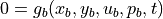
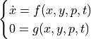
Dynamic power-system models are naturally written as differential-algebraic equations (DAEs). A standard form is [2], [3]:

$\dot{x} = f(x, y, p, t)$

$0 = g(x, y, p, t)$

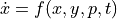
Where:

$x$ are the differential or state variables,
$y$ are the algebraic variables,
$p$ are parameters,
$t$ is time.

The differential equations describe dynamic storage and control dynamics. The algebraic equations describe instantaneous constraints such as current balance, voltage relations, or constitutive network equations.

This structure appears naturally in power systems because electrical networks impose instantaneous constraints, while machines, controllers, magnetic circuits, and energy-storage devices contribute state dynamics.

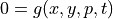
More generally, one may write the DAE in implicit form as:

$F(\dot{x},x,y,t)=0$

or, in the widely used semi-explicit form,

$\begin{cases} \dot{x} = f(x,y,t) \\ 0 = g(x,y,t) \end{cases}$

The semi-explicit form is especially useful in power systems because the distinction between dynamic and algebraic quantities is physically meaningful.

The differential part models stored energy and control memory.
The algebraic part models instantaneous network balance and constitutive constraints.

For example, synchronous-machine mechanical dynamics, controller integrators, flux dynamics, and dc-link states belong naturally to the differential part. Bus voltage relations, current-balance equations, load constitutive equations, and static network coupling belong naturally to the algebraic part.

This is why power systems are not, in general, pure ODE systems. The electrical network enforces constraints that must hold at every instant, and those constraints must be solved together with the dynamic equations.

Linearized DAE around one operating point

Let $(x^*, y^*)$ be one equilibrium point. Linearizing the semi-explicit DAE gives:

$\Delta \dot{x} = f_x \Delta x + f_y \Delta y$

$0 = g_x \Delta x + g_y \Delta y$

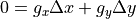
where the Jacobian submatrices are evaluated at the equilibrium point.

If $g_y$ is nonsingular, then:

$\Delta y = -g_y^{-1} g_x \Delta x$

and substitution yields the reduced state matrix:

$\Delta \dot{x} = \left(f_x - f_y g_y^{-1} g_x\right) \Delta x$

This reduced matrix is one of the foundations of eigenvalue-based small-signal analysis. It is also a strong reason to keep the nonlinear model formulation coherent: if the original DAE is inconsistent, the linearized model will be inconsistent as well.

DAE index and numerical implications

Not all DAEs are equally easy to solve. In the practical context of power-system simulation, the most desirable formulations are those that behave like index-1 DAEs, meaning that the algebraic constraints can be enforced without repeated symbolic differentiation of the algebraic equations [2], [3], [12].

This matters numerically because:

higher-index systems are harder to initialize,
Newton iterations become more fragile,
consistency conditions become more restrictive,
the solver may need additional reformulation or regularization.

This is one of the reasons why initialization, symbolic structure, and solver design cannot be documented independently. They are all aspects of the same mathematical problem.

Milano’s Power System Modelling and Scripting and Power System Modelling and Stability Analysis provide excellent references for this formulation in power-system dynamics [2], [3].

From blocks to equations in VeraGrid

In VeraGrid, each dynamic component is represented as a block. A block contains variables, equations, parameters, initialization information, and connectivity information. A complete RMS or EMT simulation model is obtained by assembling the blocks of all devices and connecting them through bus and branch interfaces.

At runtime, VeraGrid builds one global problem from those blocks:

devices contribute local equations,
buses and branches connect device ports,
event-enabled parameters are promoted to runtime values when needed,
the final problem is initialized and integrated in time.

This is conceptually the same modelling workflow described in modern equation-based dynamic simulation tools, but adapted to the grid-modelling workflow of VeraGrid.

Symbolic-numeric approach

VeraGrid uses a symbolic-numeric approach for dynamic simulation.

The idea is the following:

Models are built symbolically as blocks, equations, and variable relationships.
The symbolic structure is then assembled into one numerical problem.
Numerical solvers use the assembled equations and Jacobians to initialize and integrate the system.

This approach is used because it combines flexibility and performance:

It is easier to build reusable templates for generators, converters, loads, lines, and controllers.
It makes GUI model editing and scripting workflows consistent.
It supports automatic construction of initialization equations.
It enables structural analysis and different solver backends.
It allows parameters to be promoted to runtime event variables when needed.

In other words, VeraGrid does not hard-code one monolithic set of equations per study type. Instead, it composes the problem from modular symbolic blocks and then solves the assembled numerical system.

General idea

The symbolic-numeric approach separates model definition from numerical evaluation.

At the symbolic level, the user or template author defines:

variables,
constants,
operators,
equations,
initialization expressions,
interconnections between blocks.

At the numerical level, VeraGrid assembles those symbolic objects into evaluators, residual vectors, Jacobians, initialization problems, and time-stepping routines.

The same mathematical model can therefore be reused for:

time-domain simulation,
initialization,
linearization,
sensitivity analysis,
GUI model editing,
scripting-based workflows.

Why this matters in power systems

Power-system dynamic models are increasingly heterogeneous. Classical synchronous-machine models coexist with converter controls, custom load models, plant controllers, EMT companion models, and event-driven logic. A symbolic-numeric framework helps maintain consistency across this diversity.

The main benefits are:

explicit analytical traceability from model equations to numerical routines,
easier extension with new device templates,
exact or structurally consistent Jacobian assembly,
reduced duplication between nonlinear and linearized models,
better support for debugging and validation.

This is particularly valuable for research and development platforms such as VeraGrid, where transparency and extensibility are as important as raw numerical performance.

Symbolic models and numerical assembly

Conceptually, VeraGrid follows this sequence:

represent each device as a symbolic block,
connect the blocks into one complete network model,
identify differential variables, algebraic variables, and runtime parameters,
compile residual and Jacobian evaluators,
initialize the model,
solve the dynamic problem in time.

This architecture is what allows one RMS model or one EMT model to be both editable and solvable within the same framework.

Dynamic blocks in VeraGrid

The Block object is the central building unit for RMS and EMT models.

It can be understood as the symbolic container of one device model or one subsystem. In the same way that one mathematical model is usually written as a set of variables, equations, parameters, and constraints, a VeraGrid block stores exactly those ingredients in a structured way.

From an engineering point of view, a block is the unit that allows VeraGrid to answer all of the following questions consistently:

What are the unknown variables of this device?
Which of them are dynamic states and which are algebraic quantities?
Which equations define the model during simulation?
Which equations define the model during initialization?
Which quantities can be changed by events?
Which ports connect this model to the grid or to other submodels?

This is why the block abstraction is so important. It is not only a programming detail. It is the bridge between the physical device and the final numerical problem.

What a block contains

A block may include:

state_vars: differential state variables.
state_eqs: equations associated with those states.
algebraic_vars: algebraic variables.
algebraic_eqs: algebraic equations.
differential_eqs: explicit differential-form equations when required by the formulation.
parameters: constant block parameters.
init_values: direct initialization values.
init_eqs: initialization equations.
diff_init_eqs: initialization equations for differential quantities.
children: nested or composite blocks.

This structure allows simple components and composite templates to share the same representation.

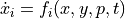
Differential and algebraic structure inside one block

At the mathematical level, a block contributes one local set of equations of the form:

$\dot{x}_b = f_b(x_b, y_b, u_b, p_b, t)$

$0 = g_b(x_b, y_b, u_b, p_b, t)$

where the subscript $b$ indicates that the variables belong to one given block. When many blocks are assembled, the global system is obtained by stacking all local equations and adding the connectivity constraints imposed by the network.

This is why a block stores both the variables and the equations. The solver does not see a visual diagram; it sees one local symbolic DAE contribution that will become part of the global system.

`state_vars` and `state_eqs`

state_vars contain the dynamic variables that represent stored energy, memory, or inertia. Examples include:

rotor angle,
rotor speed,
controller integrator states,
fluxes,
dc-link quantities,
internal dynamic references.

Their associated equations in state_eqs or, depending on formulation, in differential_eqs, describe how those states evolve in time.

In continuous time, they typically correspond to equations such as:

$\dot{x}_i = f_i(x,y,p,t)$

These are the equations that become discretized by the RMS or EMT integration method.

`algebraic_vars` and `algebraic_eqs`

algebraic_vars contain the unknowns that must satisfy instantaneous constraints. These may include:

bus voltages,
current components,
torque balances written algebraically,
power balance expressions,
converter modulation variables,
Norton-equivalent current quantities.

Their associated equations in algebraic_eqs take the generic form:

$0 = g_i(x,y,p,t)$

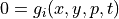
These equations are not integrated in time in the same way as states. Instead, they must be satisfied at every time step together with the discretized differential equations.

`differential_eqs` and formulation flexibility

VeraGrid supports more than one internal way of representing dynamics. In some templates, the model is naturally expressed through state equations tied to declared state variables. In others, the dynamic contribution is stored using differential_eqs explicitly.

This flexibility is useful because RMS and EMT models are not always written most naturally in the same equation form. For example:

one RMS model may be easiest to express through classical state equations,
one EMT device may be easier to express through explicitly declared derivative relations and additional algebraic couplings.

The important point is that, regardless of internal representation, the final assembled problem still corresponds to one symbolic dynamic model consistent with the solver expectations.

`parameters`

parameters store fixed constants of the model. Typical examples are:

resistances,
reactances,
inductances,
capacitances,
controller gains,
time constants,
base values,
transformer ratios,
damping and inertia constants.

Mathematically, these are the entries of the parameter vector $p$ . They define the model behavior but are not solved for during the simulation.

It is useful to distinguish them from runtime event parameters: a constant parameter remains fixed during the simulation unless it has been promoted to the runtime event structure.

`init_values`, `init_eqs`, and `diff_init_eqs`

These fields are the block’s initialization language.

init_values provide direct initial guesses or direct assigned values.
init_eqs provide symbolic equations used to reconstruct one consistent initialization point.
diff_init_eqs provide initialization expressions associated with differential quantities.

This is especially important in power-system simulation because the dynamic model is rarely initialized by simply setting all states to zero. Instead, the initialization equations tell VeraGrid how the internal variables of the device relate to the known operating point.

For example, in a synchronous-machine-type model, initialization equations may reconstruct dq currents, torque, fluxes, or references from:

power-flow voltage,
active and reactive power,
known parameters,
reference frequency.

`children` and recursive composition

The field children allows hierarchical or composite modelling. One block may contain several sub-blocks, each with its own variables and equations.

This is fundamental for composite devices. A complete generator, for instance, may be built from:

one machine block,
one exciter block,
one governor block,
one stabilizer block.

Similarly, one EMT converter may be built from:

bridge equations,
filter equations,
control logic,
modulation subsystem,
measurement or reference-conditioning blocks.

Recursive composition lets VeraGrid flatten or assemble complex devices while preserving the analytical meaning of the model.

Inputs and outputs

Dynamic connectivity is described with:

in_vars: input variables expected from other blocks.
out_vars: output variables exposed to other blocks.

During model assembly, these variables are connected by the grid variable factory, either explicitly or through helper functions such as connect_models(), connect_models_power_flow(), and the RMS/EMT bus-connection helpers.

These ports are what turn isolated symbolic models into a network model.

At the local level, one block may define equations involving some internal variables and some external quantities. Those external quantities are represented through in_vars. Once the block is connected, the inputs are matched to outputs of other blocks or to bus-shell variables.

The output variables exposed through out_vars are the quantities that the rest of the system can consume. This is how one generator can inject active and reactive power into one bus model, or how one bus can expose voltages to one branch or injection model.

RMS port logic

In RMS models, the most common coupling is through electrical operating-point variables such as:

voltage magnitude,
voltage angle,
active power,
reactive power,
branch-end quantities for from and to terminals.

The port matching is therefore often tied to power-flow-style references. This is why helper functions such as connect_models_power_flow() and bus RMS initialization helpers play an important role in the assembly process.

EMT port logic

In EMT models, ports are usually phase-domain quantities. Instead of one phasor magnitude and angle, the model may expose and consume:

phase A voltage,
phase B voltage,
phase C voltage,
neutral voltage,
phase currents,
dq-transformed internal variables depending on the model.

This makes EMT connectivity richer and also more delicate. The solver must preserve phase consistency, conductor ordering, and correct bus-shell creation for the connected devices.

`event_dict`

event_dict stores parameters or expressions that can be modified during simulation by events. This is the mechanism that allows step or ramp actions to change model parameters at runtime.

Typical uses are:

changing a load set-point,
changing a converter reference,
modifying a controller gain or source amplitude,
applying test disturbances.

This deserves emphasis because not every parameter in a dynamic model should be event-driven. A static parameter such as one inductance or one inertia constant is usually part of parameters. A runtime-adjustable set-point or disturbance-facing reference belongs conceptually to the event-enabled parameter layer.

In other words:

parameters define the device,
event_dict defines what the simulation may perturb.

That distinction is important both numerically and conceptually. It avoids confusing the permanent identity of the model with the temporary actions applied during one test scenario.

Events and promoted runtime parameters

When one parameter is placed in event_dict, VeraGrid can promote it into the runtime event structure of the global simulation problem. This allows:

step changes,
ramps,
scenario-specific parameter values,
GUI event-group workflows,
scripting-based disturbance injection.

This mechanism is one of the reasons the symbolic block formulation works well for dynamic studies: the equations do not need to be rebuilt for every disturbance scenario. Only the runtime values of the promoted parameters change.

`external_mapping`

external_mapping relates dynamic block variables to static power-flow references. This is important for consistent initialization because the dynamic model must inherit active power, reactive power, voltage magnitude, voltage angle, or analogous quantities from the solved static network.

In practical terms, external_mapping answers questions such as:

Which block variable corresponds to the active power used in the static model?
Which internal variable should receive the bus voltage magnitude from the power-flow result?
Which reactive-power or voltage-control quantity is tied to the external operating point?

This mapping is essential because the static grid objects and the dynamic block objects are not the same thing, even if they represent the same physical device. The mapping is what lets one steady-state solution initialize the correct symbolic variables inside the dynamic model.

Without this bridge, RMS dynamic simulation and small-signal linearization would lose their physical operating-point consistency.

`api_obj_mapping`

api_obj_mapping relates block parameters to API object properties. This allows a static API object, such as a generator or load, to feed parameters into the associated dynamic block.

This mapping is device-centric rather than operating-point-centric.

While external_mapping answers “which dynamic quantities correspond to the solved network state?”, api_obj_mapping answers “which dynamic block parameters correspond to the properties of the API object that owns this model?”

For example, if the static API object stores one reactance, nominal power, gain, or resistance, the dynamic block can receive that information through the API-object mapping layer. This reduces duplication and keeps the symbolic template attached to the device data model.

Composite templates

VeraGrid supports both simple and composite templates. For example:

a simple load or line template may correspond to one block,
a complete generator model may be composed of machine, exciter, governor, and stabilizer blocks,
an EMT converter model may be composed of bridge, filter, control, and modulation blocks.

This template-based workflow is one of the main advantages of the symbolic model representation.

Templates versus manual block construction

VeraGrid supports two complementary ways of building models:

use one predefined template,
build or edit the model block by block.

Templates are convenient because they package one validated structure and its initialization logic. Manual block construction is powerful because it allows custom research or development workflows.

The two approaches are not conceptually different. A template is just one preassembled symbolic block structure. The model editor exposes that same structure visually.

How blocks become one global simulation problem

Once the blocks of all devices have been assigned and connected, VeraGrid assembles the global system by:

collecting all differential variables,
collecting all algebraic variables,
collecting all parameters and event-enabled runtime parameters,
flattening composite structures when needed,
building the residual equations for the whole system,
constructing the initialization and simulation evaluators.

Symbolically, the final system looks like:

$\dot{X} = F(X,Y,P,t)$

$0 = G(X,Y,P,t)$

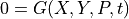
but internally this global pair $(F,G)$ is built from many local block contributions.

This local-to-global assembly is the core idea behind VeraGrid’s dynamic framework.

Initialization

Initialization is one of the most important parts of any dynamic simulation.

The objective is to compute one consistent starting point such that:

the algebraic equations are satisfied,
the state variables are consistent with the operating point,
event-enabled parameters are initialized correctly,
the simulation starts from a valid equilibrium or near-equilibrium condition.

Without this step, time integration may diverge immediately or produce physically meaningless transients.

Power flow as starting point

For RMS simulations, the standard workflow is to solve a power flow first and then use that operating point to initialize the dynamic model. This is also the workflow used by VeraGrid’s RMS dynamic and RMS small-signal drivers.

For EMT simulations, a static operating point is also needed, but the dynamic initialization problem is richer because phase-domain or waveform-domain quantities may have to be reconstructed consistently from the static network state and from model-specific initialization equations.

Initialization methods available in VeraGrid

Explicit initialization

In explicit initialization, the block templates provide enough initialization equations or direct initialization values to build the initial state from the known operating point. This is the simplest and fastest method when the model has been designed with a complete and well-conditioned initialization structure.

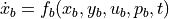
The idea is classical in DAE-based power-system simulation [2], [3]. Assume the dynamic model is written as

$\begin{cases} \dot{x} = f(x,y,p,t) \\ 0 = g(x,y,p,t) \end{cases}$

At steady state, the differential variables must satisfy equilibrium conditions, so the initialization problem becomes:

$\begin{cases} 0 = f(x_0,y_0,p,0) \\ 0 = g(x_0,y_0,p,0) \end{cases}$

The role of explicit initialization is to solve this problem not by a generic equilibrium search from scratch, but by exploiting model structure.

In practice, VeraGrid uses three sources of information:

the static network operating point, usually from power flow,
block initialization equations such as init_eqs and diff_init_eqs,
direct parameter and initial-value assignments declared by the templates.

For many RMS models, part of the variables can be filled directly from the power-flow results. Typical examples are:

bus voltage magnitude and angle,
active and reactive power injections,
branch terminal voltage quantities,
control references derived from the operating point.

After that, the remaining variables are solved using the block initialization equations. In other words, the symbolic model defines an auxiliary initialization problem where known variables are seeded from the network solution and unknown variables are reconstructed from explicit formulas or dependency-ordered equations.

At the algorithmic level, the RMS explicit initialization workflow in VeraGrid follows this philosophy:

Collect initialization equations from the system block and its children.
Collect runtime event-enabled parameters that already have known values.
Seed all variables that come directly from the solved operating point.
Build a dependency graph between initialization expressions.
Solve the initialization equations in topological order whenever possible.
Use a local nonlinear solve only for the variables that cannot be assigned directly by substitution.

This is why explicit initialization is usually the fastest option: it reuses as much analytical structure as possible instead of treating initialization as one black-box nonlinear problem.

From a modelling perspective, explicit initialization works best when the template designer has written initialization equations that are:

complete,
non-circular or weakly circular,
physically meaningful,
consistent with the static operating point.

This is especially natural for RMS phasor-domain models, where many electrical quantities already have clear steady-state interpretations.

Use it when:

the templates already provide a robust initialization path,
the model is not heavily implicit at initialization,
you want the most direct workflow.

Pseudo-transient initialization

Pseudo-transient continuation is a robust technique for finding equilibria of DAEs by integrating an artificial transient until the residual becomes small [2], [3]. VeraGrid uses pseudo-transient initialization as an alternative when explicit initialization is insufficient or too fragile.

Suppose the equilibrium problem is written compactly as:

$F(z)=0$

where $z$ groups the unknown initialization quantities. A direct Newton solve may fail if:

the initial guess is poor,
the Jacobian is ill-conditioned,
the system is strongly nonlinear,
some controls interact too tightly,
the model is only partially initialized by explicit formulas.

Pseudo-transient continuation addresses this by embedding the equilibrium problem in an artificial dynamic process:

$M \frac{dz}{d\tau} = -F(z)$

where:

$\tau$ is an artificial continuation time,
$M$ is a scaling or pseudo-mass matrix,
the steady state of this artificial system satisfies the original equilibrium condition $F(z)=0$ .

The intuition is simple: instead of asking Newton to jump directly to the equilibrium, the method lets the residual decay progressively. This greatly improves robustness for badly conditioned or weakly initialized systems.

In one backward-Euler pseudo-transient step, the update has the generic form:

$M\frac{z^{k+1}-z^k}{\Delta \tau_k} + F(z^{k+1}) = 0$

which can be interpreted as a sequence of regularized nonlinear solves. When $\Delta \tau_k$ is small, the method behaves conservatively and is robust. As the residual becomes better behaved, $\Delta \tau_k$ can be increased so the method approaches the final equilibrium more aggressively.

This is one of the reasons pseudo-transient continuation is widely appreciated in power-system DAE solving: it acts as a bridge between time integration and nonlinear equilibrium solving [2], [3], [12].

How VeraGrid uses pseudo-transient initialization

In VeraGrid, pseudo-transient initialization is not only a theoretical option. It is part of the live RMS and EMT initialization stack.

For RMS, the pseudo-transient workflow is used when the equilibrium cannot be recovered robustly through explicit initialization alone. The solver builds one numerical problem from the symbolic dynamic model, seeds the unknown vector with available initialization values and operating-point information, and then runs one pseudo-transient relaxation process. After that, VeraGrid performs a Newton polishing stage to reduce the final residual further.

This means the practical RMS initialization sequence is roughly:

build one initial guess from the available initialization map,
enforce critical references or seeded quantities when needed,
run pseudo-transient relaxation,
refine the solution with Newton iterations,
verify the final residual before accepting the initialization.

For EMT, the same philosophy is used but adapted to the EMT problem structure. VeraGrid builds a reduced initialization system for the unresolved EMT variables and then applies a pseudo-transient solve to that reduced system. This is particularly useful because EMT initialization may involve:

reconstructed phase-domain voltages and currents,
internal device states such as dq fluxes or machine states,
algebraic constraints from phase-domain network coupling,
missing derivative initial values that must be completed consistently.

The EMT initialization code therefore uses pseudo-transient continuation as one robust fallback or selected workflow to recover a consistent initial condition for the waveform-domain model.

Why pseudo-transient is so useful in dynamic simulation

Pseudo-transient continuation is especially effective when the initialization problem is stiff or poorly scaled. In power-system terms, this often happens when:

the network constraints and control equations are tightly coupled,
converter-rich systems create weakly damped algebraic interactions,
device references are not perfectly matched to the power-flow operating point,
some state variables are missing direct explicit formulas.

Instead of failing immediately, the pseudo-transient process gives the model a numerically controlled way to settle into equilibrium.

Use it when:

explicit initialization fails,
the system is strongly nonlinear,
a better basin of attraction is needed for the equilibrium solution,
the model contains tightly coupled controls or implicit algebraic relations.

In VeraGrid, the pseudo-transient workflow is implemented both in RMS and in EMT initialization logic, with EMT using a reduced initialization system adapted to the EMT formulation.

Practical recommendation

Start with Explicit when the model is known to initialize well.
Switch to PseudoTransient when the model is difficult to initialize or when explicit initialization becomes fragile.

As a practical engineering rule:

choose Explicit when the template has a clean and well-defined steady-state construction,
choose PseudoTransient when the model is implicit, strongly coupled, or still under development,
inspect initialization residuals whenever the first simulation samples look suspicious.

Typical symptoms of bad initialization are:

nonphysical spikes at the first steps,
immediate divergence of Newton iterations,
states starting far from their expected operating region,
algebraic variables inconsistent with the power-flow operating point,
large initial residual norms.

Initialization references

The theoretical background for the DAE equilibrium problem and pseudo-transient continuation is discussed in [2], [3], [12]. For EMT initialization in converter-rich and power-electronics-dominated systems, additional practical considerations can be found in [6] and in recent EMT initialization literature [7].

Solvers and integration methods

RMS solvers and integration methods

The current RMS workflow is driven through RmsOptions and RmsSimulationDriver.

RMS options include:

integration_method
initialization_method
problem_type
time_step
simulation_time
tolerance
use_init_values
max_iter

The main user-facing RMS integration method currently exposed in the driver workflow is:

DAE Backward Euler (DynamicIntegrationMethod.DaeBackEuler)

Backward Euler is a classical robust implicit method for stiff DAEs and is widely used in transient-stability and dynamic-simulation contexts [1]-[3].

For one differential equation

$\dot{x}=f(x,t)$

the backward Euler discretization is:

$x_{k+1}=x_k+h f(x_{k+1}, t_{k+1})$

This is implicit because the future state appears on the right-hand side. In a DAE system, the update is not solved variable by variable, but as one coupled nonlinear problem involving both the discretized differential equations and the algebraic constraints.

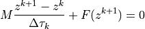
For a semi-explicit DAE,

$\begin{cases} \dot{x}=f(x,y) \\ 0=g(x,y) \end{cases}$

backward Euler leads to:

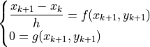
$\begin{cases} \dfrac{x_{k+1}-x_k}{h} = f(x_{k+1}, y_{k+1}) \\ 0=g(x_{k+1}, y_{k+1}) \end{cases}$

The solver must therefore compute $(x_{k+1}, y_{k+1})$ simultaneously, usually through Newton iterations.

The advantages of backward Euler in RMS simulation are:

strong numerical robustness,
good behavior for stiff electromechanical-control systems,
compatibility with implicit DAE formulations,
reasonable performance with relatively large time steps.

Its drawbacks are also classical:

first-order accuracy,
numerical damping,
the need for nonlinear solves at each step.

In RMS transient-stability work, this trade-off is usually acceptable because the main interest is robust evolution of relatively slow variables rather than highly accurate waveform reconstruction.

EMT solvers and integration methods

The EMT workflow is driven through EmtOptions and EmtSimulationDriver.

EMT options include:

solver_type
integration_method
initialization_method
problem_type
time_step
simulation_time
tolerance
initialization Newton and pseudo-transient settings
sparse-solver and Newton diagnostics options

The default EMT integration method is:

DAE Trapezoidal (DynamicIntegrationMethod.DaeTrapezoidal)

This is consistent with standard EMTP practice, where trapezoidal integration is a classical default because of its accuracy and energy behavior for network transients [4]-[6].

For one generic state equation,

$\dot{x}=f(x,t)$

the trapezoidal discretization is:

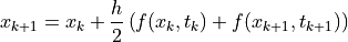
$x_{k+1}=x_k+\frac{h}{2}\left(f(x_k,t_k)+f(x_{k+1},t_{k+1})\right)$

This is again an implicit method, but of second order. In EMT simulation, trapezoidal integration is especially powerful because passive elements can be rewritten as companion models.

For example, an inductance described by

$v=L\frac{di}{dt}$

can be discretized into one equivalent Norton or Thevenin form containing:

one equivalent conductance or resistance,
one history term that depends on the previous step.

The same logic applies to capacitors, RLC loads, several transformer models, and line companion models. This is the numerical heart of the classical Dommel EMTP approach [4], [5].

EMT solver backends

Beyond the integration method itself, VeraGrid’s EMT workflow supports different solver backends through EmtSolverTypes. These backends correspond to different ways of assembling and solving the EMT equations while keeping the same general simulation objective.

At a user level, the important point is:

the physics is still EMT waveform-domain simulation,
the backend changes how the equations are assembled and solved,
different backends may offer different trade-offs between transparency, flexibility, and speed.

Choosing time step, method, and backend

The time step and solver configuration must be coherent with the phenomenon under study.

In practice:

RMS usually tolerates millisecond-order steps because the focus is on slower dynamics,
EMT usually requires microsecond-order steps because the solver must resolve fast electrical transients,
explicit switching models or travelling-wave models may force even smaller EMT steps,
weakly initialized or very stiff systems may require more robust solver settings.

The best choice is therefore not universal. It depends on the model bandwidth, the event speed, the line delays, and the degree of detail requested by the study.

The EMT driver can use different solver backends depending on the configured EmtSolverTypes, which allows users to trade development flexibility, structural exploitation, and runtime performance.

Choosing time step and domain

As a practical rule:

RMS time steps are usually in the order of milliseconds.
EMT time steps are usually in the order of microseconds or smaller.

If the chosen time step is too large, the simulation may miss important dynamics or fail to converge. If it is too small, the simulation may become unnecessarily expensive.

Events and simulation scenarios

Dynamic studies are usually meaningful only when some disturbance or scheduled action is applied.

In VeraGrid, events are organized in two layers:

Event groups: one scenario or simulation case.
Events: the actual runtime parameter changes applied during that scenario.

Both RMS and EMT support event groups and runtime parameter modification.

Typical event types are:

Step events.
Ramp events.

Examples include:

changing Pl0 of a load,
changing a reference voltage,
changing a converter power command,
changing source amplitude or frequency.

Each active event group produces one trajectory set in the results object.

Settings

RMS settings

The RMS settings exposed through RmsOptions are:

Integration method: numerical integration method. In the current driver workflow the standard method is DaeBackEuler.
Initialization method: initialization workflow, mainly Explicit or PseudoTransient.
Problem type: internal RMS problem formulation.
Time step (s): interval between numerical integration steps.
Simulation time (s): final simulation time.
Tolerance: numerical tolerance used by the simulation workflow.
Use init values: whether stored initialization values should be reused when available.
Max. iterations: maximum number of nonlinear iterations inside the solver.

EMT settings

The EMT settings exposed through EmtOptions are:

Solver type: EMT backend to use.
Integration method: default DaeTrapezoidal.
Initialization method: EMT initialization workflow.
Problem type: internal EMT problem formulation.
Time step (s): EMT integration step.
Simulation time (s): total EMT simulation horizon.
Tolerance: numerical tolerance.
Initialization Newton controls: tolerances, iteration limits, and backtracking.
Pseudo-transient controls: init_ptc_dtau0, init_ptc_dtau_min, init_ptc_dtau_max, init_ptc_max_iter.
Sparse-solver controls: sparse solver selection and fallback behavior.
Newton diagnostics and stabilization controls: backtracking, fallback, index checks, conditioning diagnostics.

For most users, only solver type, initialization method, integration method, time step, simulation time, and tolerance need to be changed regularly. The other parameters are advanced controls.

Results

RMS results

The RMS dynamic results are stored in RmsResults.

Main registered properties include:

time_array: simulation time stamps.
values: simulated variable values.
rms_events_group_names: names of declared RMS event groups.
rms_events_group_idtags: identifiers of declared RMS event groups.
has_event_group_results: mask of groups that actually produced results.
well_initialized: initialization status per event group.
converged: convergence status per event group.
dynamic_metadata_json: serialized metadata for variable recovery and plotting.

EMT results

The EMT dynamic results are stored in EmtResults.

Main registered properties include:

time_array: simulation time stamps.
values: simulated state and algebraic variable values.
diff_values: differential-variable trajectories.
emt_events_group_names: names of declared EMT event groups.
emt_events_group_idtags: identifiers of declared EMT event groups.
has_event_group_results: mask of groups that actually produced results.
well_initialized: initialization status per event group.
converged: convergence status per event group.
dynamic_metadata_json: serialized metadata for variable recovery and plotting.

API workflow overview

The general scripting workflow for dynamic simulations in VeraGrid is:

Build or load the static grid.
Assign RMS or EMT dynamic models to the devices.
Run the required power flow.
Create event groups and events if needed.
Define the simulation options.
Run the corresponding driver.
Read the results arrays and post-process the trajectories.

RMS example from scripting

The following example shows the current RMS scripting workflow using templates and the RMS driver.

from VeraGridEngine.Devices.Substation.bus import Bus
from VeraGridEngine.Devices.Injections.generator import Generator
from VeraGridEngine.Devices.Injections.load import Load
from VeraGridEngine.Devices.Branches.line import Line

from VeraGridEngine.enumerations import DynamicIntegrationMethod, RmsInitializationMethod
from VeraGridEngine.Templates.Rms.genqec_exc_gov_sat_template_v2 import get_complete_generator_template_rms
from VeraGridEngine.Templates.Rms.line_rms_template import get_line_rms_template
from VeraGridEngine.Templates.Rms.load_rms_template import get_load_rms_template
from VeraGridEngine.Utils.Symbolic.bus_rms_template import initialize_bus_rms
from VeraGridEngine.Utils.Symbolic.templates_common_functions import set_rms_model

from VeraGridEngine.Simulations.PowerFlow.power_flow_driver import PowerFlowOptions
from VeraGridEngine.Simulations.Rms.rms_options import RmsOptions
from VeraGridEngine.Simulations.Rms.rms_driver import RmsSimulationDriver

import VeraGridEngine.api as gce

grid = gce.MultiCircuit(Sbase=100.0, fbase=50.0)

bus0 = Bus(name="Bus0", Vnom=10.0, is_slack=True)
bus1 = Bus(name="Bus1", Vnom=10.0)
grid.add_bus(bus0)
grid.add_bus(bus1)

for bus in grid.buses:
    initialize_bus_rms(bus, vf=grid.var_factory)

line = gce.Line(name="line 0-1", bus_from=bus0, bus_to=bus1, r=0.029585, x=0.071005, b=0.03, rate=900.0)
grid.add_line(line)

load = gce.Load(name="Load1", P=9.999999, Q=0.999999)
grid.add_load(bus=bus1, api_obj=load)

gen = Generator(name="Gen0", P=10.0, vset=1.0, Snom=900.0, x1=0.86138701, r1=0.3, freq=50.0)
grid.add_generator(bus=bus0, api_obj=gen)

# Build and assign RMS templates
gen_rms = get_complete_generator_template_rms(grid.var_factory).block
line_rms = get_line_rms_template(grid.var_factory).block
load_rms = get_load_rms_template(grid.var_factory).block

set_rms_model(device=gen, model=gen_rms, var_factory=grid.var_factory)
set_rms_model(device=line, model=line_rms, var_factory=grid.var_factory)
set_rms_model(device=load, model=load_rms, var_factory=grid.var_factory)

# Change one runtime parameter from the API side
load.rms_model.set_parameter_in_model(var_name="Pl0", new_value=-0.10)

pf_options = PowerFlowOptions(solver_type=gce.SolverType.NR, verbose=0)
pf_results = gce.power_flow(grid, options=pf_options)

rms_options = RmsOptions(
    time_step=0.001,
    simulation_time=1.0,
    tolerance=1e-6,
    integration_method=DynamicIntegrationMethod.DaeBackEuler,
    initialization_method=RmsInitializationMethod.Explicit,
    use_init_values=False,
    max_iter=1000,
    verbose=0,
)

driver = RmsSimulationDriver(grid=grid, options=rms_options, pf_results=pf_results)
driver.run()

results = driver.results
print(results.converged)
print(results.well_initialized)
print(results.values.shape)

This example illustrates the main RMS workflow:

initialize RMS bus shells,
assign RMS templates,
connect them through set_rms_model(),
update parameters,
run power flow,
run RmsSimulationDriver,
inspect RmsResults.

EMT example from scripting

The following example shows the current EMT workflow structure. EMT examples in VeraGrid are typically more detailed because they often use phase-domain devices, line templates, and solver backends.

from VeraGridEngine.Devices.Substation.bus import Bus
from VeraGridEngine.Devices.Injections.generator import Generator
from VeraGridEngine.Devices.Injections.load import Load
from VeraGridEngine.Devices.Branches.line import Line

from VeraGridEngine.enumerations import DynamicIntegrationMethod, EmtInitializationMethod, EmtSolverTypes
from VeraGridEngine.Templates.Emt.pi_line_emt_template import get_pi_line_emt_template
from VeraGridEngine.Templates.Emt.thevenin_equivalent_emt_generator_template import (
    get_generator_thevenin_rl_emt_template_with_ref,
)
from VeraGridEngine.Templates.Emt.load_RLC_emt_template import get_shunt_r_emt_template
from VeraGridEngine.Utils.Symbolic.templates_common_functions import set_emt_model

from VeraGridEngine.Simulations.PowerFlow.power_flow_driver import PowerFlowOptions
from VeraGridEngine.Simulations.EMT.emt_options import EmtOptions
from VeraGridEngine.Simulations.EMT.emt_driver import EmtSimulationDriver

import VeraGridEngine.api as gce

grid = gce.MultiCircuit(Sbase=100.0, fbase=50.0)

bus0 = Bus(name="Bus0", Vnom=10.0, is_slack=True)
bus1 = Bus(name="Bus1", Vnom=10.0)
grid.add_bus(bus0)
grid.add_bus(bus1)

line = Line(name="line 0-1", bus_from=bus0, bus_to=bus1, r=0.02, x=0.08, b=0.0, rate=100.0)
grid.add_line(line)

gen = Generator(name="Gen1", P=1.0, vset=1.0, Snom=100.0, r1=0.001, x1=1.7)
grid.add_generator(bus=bus0, api_obj=gen)

load = Load(name="Load1", P=1.0, Q=0.0)
grid.add_load(bus=bus1, api_obj=load)

# Build and assign EMT templates
gen_emt = get_generator_thevenin_rl_emt_template_with_ref(grid.var_factory).block
line_emt = get_pi_line_emt_template(
    vf=grid.var_factory,
    phN=False,
    phA=True,
    phB=True,
    phC=True,
).block
load_emt = get_shunt_r_emt_template(
    vf=grid.var_factory,
    phA=True,
    phB=True,
    phC=True,
).block

set_emt_model(device=gen, model=gen_emt, var_factory=grid.var_factory)
set_emt_model(device=line, model=line_emt, var_factory=grid.var_factory)
set_emt_model(device=load, model=load_emt, var_factory=grid.var_factory)

# Change one EMT parameter from the API side
load.emt_model.set_parameter_in_model(var_name="R_A", new_value=200.0)

pf_options = PowerFlowOptions(solver_type=gce.SolverType.NR, verbose=0)
pf_results = gce.power_flow(grid, options=pf_options)

emt_options = EmtOptions(
    time_step=1e-6,
    simulation_time=0.02,
    tolerance=1e-6,
    solver_type=EmtSolverTypes.StructuralAD,
    integration_method=DynamicIntegrationMethod.DaeTrapezoidal,
    initialization_method=EmtInitializationMethod.Auto,
    verbose=0,
)

driver = EmtSimulationDriver(grid=grid, options=emt_options, pf_results=pf_results)
driver.run()

results = driver.results
print(results.converged)
print(results.well_initialized)
print(results.values.shape)
print(results.diff_values.shape)

This example illustrates the same general workflow as RMS, but using EMT templates, EMT options, and the EMT driver.

Working with templates and model editors

In VeraGrid there are two main ways to assign dynamic models to a device:

Assign an RMS or EMT template from the catalogue or from the device properties.
Open the RMS or EMT editor and build the model graphically from blocks.

The editor-based workflow is especially useful when:

controller parameters must be tuned,
a composite model has to be inspected,
the user wants to create or modify one template,
the structure of the block itself must be validated.

The practical RMS and EMT session documents are good companions for the GUI workflow:

RMS_practical_session.md
EMT_practical_session.md

Importing dynamic models from external tools

Dynamic-model interoperability is an important topic, but it must be described carefully because not all external modelling ecosystems map directly to VeraGrid blocks.

At the moment, the relevant VeraGrid mechanisms are:

native RMS and EMT templates,
FMU-related import and runtime support,
parameter and template assignment through the VeraGrid device model.

This means that some external dynamic models can be integrated through FMU-based workflows, while others may need to be recreated as VeraGrid templates or composite blocks.

This section should be considered an evolving area of the documentation. The exact scope of supported import workflows is still under active consolidation.

Benchmarks and validation

VeraGrid already contains validation and benchmark work for dynamic simulation in trunk, including:

RMS validation scripts in trunk/dynamics/model_validation/
pseudo-transient validation scripts in trunk/dynamics/
EMT multi-solver benchmark scripts in trunk/dynamics_emt/

However, this section is intentionally left only partially developed here because the benchmark narrative and the final comparative claims still need to be consolidated.

For now, the main point is that VeraGrid includes internal validation assets for:

RMS model behavior,
EMT backend comparison,
pseudo-transient initialization workflows,
small-system and detailed-device consistency checks.

Best practices

Solve and verify the static power flow before attempting RMS or EMT simulation.
Start with the simplest model that can answer the engineering question.
Use RMS first unless waveform or switching detail is truly required.
Use explicit initialization when the templates are known to initialize robustly.
Use pseudo-transient initialization when explicit initialization becomes fragile.
Keep time steps physically justified; smaller is not always better if the domain choice is wrong.
Validate one device model in a small test system before using it in a large case.
Attach events only to parameters intended to be modified at runtime.

Common pitfalls

Running a dynamic simulation without a valid operating point.
Using an RMS model for a phenomenon that actually requires EMT detail.
Choosing an EMT time step that is too large for switching dynamics.
Missing bus/device dynamic connections when building custom templates.
Inconsistent parameterization between static and dynamic models.
Expecting one model to initialize if the initialization equations are incomplete.

References

[1] P. Kundur, Power System Stability and Control. McGraw-Hill, 1994.

[2] F. Milano, Power System Modelling and Scripting. Springer, 2010.

[3] F. Milano, Power System Modelling and Stability Analysis. Springer, 2010.

[4] H. W. Dommel, EMTP Theory Book. Bonneville Power Administration, 1986.

[5] L. Gérin-Lajoie, J. Mahseredjian, and collaborators, EMTP-RV Theory Book. Powersys Solutions, various editions.

[6] J. Mahseredjian, V. Dinavahi, and J. A. Martinez, “Simulation Tools for Electromagnetic Transients in Power Systems: Overview and Challenges,” IEEE Transactions on Power Delivery, vol. 24, no. 3, pp. 1657-1669, 2009.