🔍 Small-Signal stability analysis
RMS Small-Signal Stability assessment is crucial for any system and of course, VeraGrid has it.
⚠️Before performing small-signal stability analysis, a power flow calculation must be completed!
Settings
This is the Small-Signal settings page:
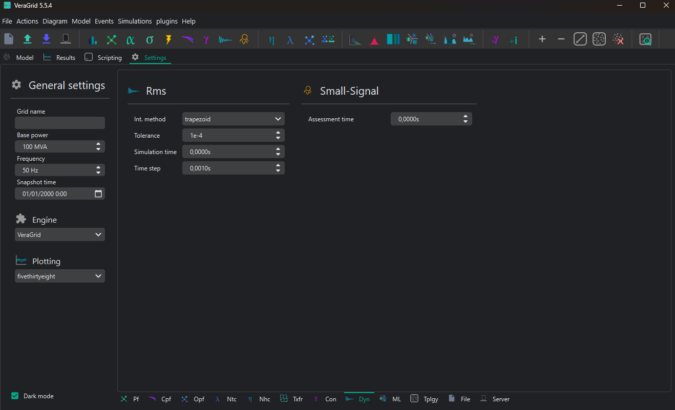
The main setting in Small-Signal Stability assessment is the time instant when the analysis is performed. Therefore, if the assessment time is zero, no dynamic simulation is needed and the only parameter to set is the assessment time itself. Otherwise, Rms dynamic simulation parameters must be considered.
Settings from Small-signal:
Assessment time (s): The time instant in seconds where the stability assessment is performed.
Settings from RMS simulations that must be considered:
Integration method: The integration method to use if the Rms dynamic simulation is performed.
Trapezoidal
Implicit euler
Tolerance: per-unit error tolerance to use in the integration method. Only needed if the Rms dynamic simulation is performed.
Time step (s): Step size in seconds between each numerical evaluation in the integration method. Smaller intervals increase accuracy but require more computation. Only needed if the Rms dynamic simulation is performed.
Results
The available results are the following:
State matrix: State matrix of the state-space representation of the system.
Modes: Table with the modes and damping ratios and oscillation frequencies of the complex conjugate modes.
Participation factors: The participation factor of variable k in mode i is found in row k, column i.
S-Domain stability plot: available with different imaginary axis units: “rad/s” or “Hz”.

Registered Result Properties
SmallSignalStabilityRmsResults registered properties
The RMS small-signal stability result stores eigenvalue, damping, frequency, participation, and state-matrix data.
Property |
Type |
Description |
|---|---|---|
|
|
Eigenvalues of the linearized system. |
|
|
Participation-factor matrix relating states or variables to modes. |
|
|
Damping ratio for each identified mode. |
|
|
Frequency of each complex-conjugate mode. |
|
|
State matrix of the linearized system. |
SmallSignalStabilityEmtResults registered properties
The EMT small-signal stability result stores multiplier, eigenvalue, and participation-factor data.
Property |
Type |
Description |
|---|---|---|
|
|
Discrete-time multipliers from the EMT small-signal analysis. |
|
|
Eigenvalues of the linearized system. |
|
|
Participation-factor matrix relating states or variables to modes. |
EraMatrixPencilResults registered properties
The ERA matrix pencil result stores modal estimates and reconstruction diagnostics.
Property |
Type |
Description |
|---|---|---|
|
|
Estimated continuous-time eigenvalues in the s-domain. |
|
|
Mode frequencies in hertz. |
|
|
Damping ratio for each identified mode. |
|
|
Stability flag for each identified mode. |
|
|
Modal residues estimated by the ERA matrix pencil method. |
|
|
Estimated energy contribution of each mode. |
|
|
Signal reconstruction error for each selected model order. |
|
|
Lower frequency bound used for modal selection. |
|
|
Upper frequency bound used for modal selection. |
|
|
Model orders selected by the ERA matrix pencil analysis. |
|
|
Number of observed signals contributing to each mode. |
RmsResults registered properties
The RMS result stores the simulated variable values.
Property |
Type |
Description |
|---|---|---|
|
|
Simulated values matrix for the registered dynamic variables. |
EmtResults registered properties
The EMT result stores the simulated variable values.
Property |
Type |
Description |
|---|---|---|
|
|
Simulated values matrix for the registered dynamic variables. |
API
Using the RMS small-signal API:
import os

from VeraGridEngine.enumerations import DynamicIntegrationMethod
from VeraGridEngine.Simulations.PowerFlow.power_flow_driver import PowerFlowOptions, PowerFlowDriver
from VeraGridEngine.Simulations.Rms.rms_options import RmsOptions
from VeraGridEngine.Simulations.SmallSignalStabilityRms.small_signal_driver import (
    SmallSignalStabilityRmsDriver,
    plot_stability,
)
from VeraGridEngine.Simulations.SmallSignalStabilityRms.small_signal_options import (
    RmsSmallSignalStabilityOptions,
)
import VeraGridEngine.api as gce

folder = os.path.join('..', 'Grids_and_profiles', 'grids')
fname = os.path.join(folder, 'IEEE39_1W.veragrid')
grid = gce.open_file(fname)

# A power flow must be available before the RMS small-signal assessment.
pf_options = PowerFlowOptions(solver_type=gce.SolverType.NR, verbose=False)
power_flow = PowerFlowDriver(grid=grid, options=pf_options)
power_flow.run()
pf_results = power_flow.results

# RMS options are only used when ss_assessment_time > 0, because the driver
# performs an RMS simulation from t=0 up to the assessment instant.
rms_options = RmsOptions(
    time_step=0.001,
    simulation_time=20.0,
    tolerance=1e-6,
    integration_method=DynamicIntegrationMethod.DaeBackEuler,
    max_iter=1000,
    verbose=0,
)

# Case 1: assessment at t = 0 s (no RMS dynamic simulation is run).
ss_options_t0 = RmsSmallSignalStabilityOptions(
    ss_assessment_time=0.0,
    k=0,
    verbose=1,
)

small_signal_t0 = SmallSignalStabilityRmsDriver(
    grid=grid,
    rms_options=rms_options,
    sss_options=ss_options_t0,
    pf_results=pf_results,
)
small_signal_t0.run_small_signal_stability()

eigenvalues_t0 = small_signal_t0.results.eigenvalues
participation_factors_t0 = small_signal_t0.results.participation_factors
damping_ratios_t0 = small_signal_t0.results.damping_ratios
conjugate_frequencies_t0 = small_signal_t0.results.conjugate_frequencies
state_matrix_t0 = small_signal_t0.results.state_matrix

# Case 2: assessment at t = 20 s.
# The driver first runs the RMS simulation and then linearizes the system at t = 20 s.
ss_options_t20 = RmsSmallSignalStabilityOptions(
    ss_assessment_time=20.0,
    k=0,
    verbose=1,
)

small_signal_t20 = SmallSignalStabilityRmsDriver(
    grid=grid,
    rms_options=rms_options,
    sss_options=ss_options_t20,
    pf_results=pf_results,
)
small_signal_t20.run_small_signal_stability()

eigenvalues_t20 = small_signal_t20.results.eigenvalues
participation_factors_t20 = small_signal_t20.results.participation_factors
damping_ratios_t20 = small_signal_t20.results.damping_ratios
conjugate_frequencies_t20 = small_signal_t20.results.conjugate_frequencies
state_matrix_t20 = small_signal_t20.results.state_matrix
Output:
Eigenvalues: [-2.+64.08943759j -2.-64.08943759j -0. +0.j         -2.+44.07988997j -2.-44.07988997j -2.+43.18166955j -2.-43.18166955j -2.+42.76559246j -2.-42.76559246j -2.+38.07928002j -2.-38.07928002j -2.+36.155124j   -2.-36.155124j   -2.+21.84445116j -2.-21.84445116j -2.+24.66622044j -2.-24.66622044j -2.+30.09976294j
 -2.-30.09976294j -2.+26.68017287j -2.-26.68017287j -4. +0.j        ]
Daming ratios: ['0.031191206336476197', '-', '-', '0.04532553372859127', '-', '0.04626635094680637', '-', '0.04671551016349282', '-', '0.05244970840548839', '-', '0.05523275243053552', '-', '0.09117508790940405', '-', '0.08081732123290178', '-', '0.06629951000786061', '-', '0.07475229922283681', '-', '-']
Oscillation frequencies[Hz]: ['10.200150792654048', '-', '-', '7.0155323802875404', '-', '6.872576160385048', '-', '6.806355434076857', '-', '6.06050564510895', '-', '5.7542667023807', '-', '3.4766523816869435', '-', '3.9257509100087766', '-', '4.790526057009294', '-', '4.246281394817547', '-', '-']
Participation factors: [[0.00357204 0.00357204 0.0926209  0.00074082 0.00074082 0.25126465 0.25126465 0.07900952 0.07900952 0.00004668 0.00004668 0.00316457 0.00316457 0.02426172 0.02426172 0.00344389 0.00344389 0.0877041  0.0877041  0.00048156 0.00048156 0.        ]
 [0.00357204 0.00357204 0.         0.00074082 0.00074082 0.25126465 0.25126465 0.07900952 0.07900952 0.00004668 0.00004668 0.00316457 0.00316457 0.02426172 0.02426172 0.00344389 0.00344389 0.0877041  0.0877041  0.00048156 0.00048156 0.0926209 ]
 [0.01426164 0.01426164 0.09238855 0.00000793 0.00000793 0.00021923 0.00021923 0.00000009 0.00000009 0.26700701 0.26700701 0.00212486 0.00212486 0.03034834 0.03034834 0.08097717 0.08097717 0.05779924 0.05779924 0.00106021 0.00106021 0.        ]
 [0.01426164 0.01426164 0.         0.00000793 0.00000793 0.00021923 0.00021923 0.00000009 0.00000009 0.26700701 0.26700701 0.00212486 0.00212486 0.03034834 0.03034834 0.08097717 0.08097717 0.05779924 0.05779924 0.00106021 0.00106021 0.09238855]
 [0.0537019  0.0537019  0.09168668 0.00010264 0.00010264 0.00001923 0.00001923 0.00393335 0.00393335 0.21081061 0.21081061 0.04664987 0.04664987 0.02012104 0.02012104 0.06597425 0.06597425 0.0523657  0.0523657  0.00047807 0.00047807 0.        ]
 [0.0537019  0.0537019  0.         0.00010264 0.00010264 0.00001923 0.00001923 0.00393335 0.00393335 0.21081061 0.21081061 0.04664987 0.04664987 0.02012104 0.02012104 0.06597425 0.06597425 0.0523657  0.0523657  0.00047807 0.00047807 0.09168668]
 [0.00297603 0.00297603 0.08976704 0.24594546 0.24594546 0.017432   0.017432   0.05843227 0.05843227 0.00002158 0.00002158 0.         0.         0.07855066 0.07855066 0.00025169 0.00025169 0.00000381 0.00000381 0.05150299 0.05150299 0.        ]
 [0.00297603 0.00297603 0.         0.24594546 0.24594546 0.017432   0.017432   0.05843227 0.05843227 0.00002158 0.00002158 0.         0.         0.07855066 0.07855066 0.00025169 0.00025169 0.00000381 0.00000381 0.05150299 0.05150299 0.08976704]
 [0.00012145 0.00012145 0.08998892 0.11268232 0.11268232 0.0120963  0.0120963  0.04981461 0.04981461 0.00048795 0.00048795 0.0004482  0.0004482  0.13621279 0.13621279 0.0005366  0.0005366  0.00001986 0.00001986 0.14258547 0.14258547 0.        ]
 [0.00012145 0.00012145 0.         0.11268232 0.11268232 0.0120963  0.0120963  0.04981461 0.04981461 0.00048795 0.00048795 0.0004482  0.0004482  0.13621279 0.13621279 0.0005366  0.0005366  0.00001986 0.00001986 0.14258547 0.14258547 0.08998892]
 [0.00355442 0.00355442 0.09056877 0.10511506 0.10511506 0.06579047 0.06579047 0.14419363 0.14419363 0.00000978 0.00000978 0.0000125  0.0000125  0.04085957 0.04085957 0.00004103 0.00004103 0.00003311 0.00003311 0.09510605 0.09510605 0.        ]
 [0.00355442 0.00355442 0.         0.10511506 0.10511506 0.06579047 0.06579047 0.14419363 0.14419363 0.00000978 0.00000978 0.0000125  0.0000125  0.04085957 0.04085957 0.00004103 0.00004103 0.00003311 0.00003311 0.09510605 0.09510605 0.09056877]
 [0.00035084 0.00035084 0.09012679 0.03523002 0.03523002 0.03866155 0.03866155 0.10979721 0.10979721 0.0008192  0.0008192  0.00084248 0.00084248 0.06252575 0.06252575 0.0000789  0.0000789  0.00011193 0.00011193 0.20651874 0.20651874 0.        ]
 [0.00035084 0.00035084 0.         0.03523002 0.03523002 0.03866155 0.03866155 0.10979721 0.10979721 0.0008192  0.0008192  0.00084248 0.00084248 0.06252575 0.06252575 0.0000789  0.0000789  0.00011193 0.00011193 0.20651874 0.20651874 0.09012679]
 [0.0004793  0.0004793  0.08902137 0.0001083  0.0001083  0.09468602 0.09468602 0.04503221 0.04503221 0.00642155 0.00642155 0.11251576 0.11251576 0.03014674 0.03014674 0.01891151 0.01891151 0.14656132 0.14656132 0.00062661 0.00062661 0.        ]
 [0.0004793  0.0004793  0.         0.0001083  0.0001083  0.09468602 0.09468602 0.04503221 0.04503221 0.00642155 0.00642155 0.11251576 0.11251576 0.03014674 0.03014674 0.01891151 0.01891151 0.14656132 0.14656132 0.00062661 0.00062661 0.08902137]
 [0.00025615 0.00025615 0.08768682 0.0000086  0.0000086  0.00001203 0.00001203 0.00021251 0.00021251 0.00001783 0.00001783 0.00482891 0.00482891 0.03369426 0.03369426 0.30064902 0.30064902 0.11624527 0.11624527 0.00023201 0.00023201 0.        ]
 [0.00025615 0.00025615 0.         0.0000086  0.0000086  0.00001203 0.00001203 0.00021251 0.00021251 0.00001783 0.00001783 0.00482891 0.00482891 0.03369426 0.03369426 0.30064902 0.30064902 0.11624527 0.11624527 0.00023201 0.00023201 0.08768682]
 [0.00322139 0.00322139 0.09364509 0.0000261  0.0000261  0.01981826 0.01981826 0.00867828 0.00867828 0.00874676 0.00874676 0.32699964 0.32699964 0.03847909 0.03847909 0.01267044 0.01267044 0.03314817 0.03314817 0.00138933 0.00138933 0.        ]
 [0.00322139 0.00322139 0.         0.0000261  0.0000261  0.01981826 0.01981826 0.00867828 0.00867828 0.00874676 0.00874676 0.32699964 0.32699964 0.03847909 0.03847909 0.01267044 0.01267044 0.03314817 0.03314817 0.00138933 0.00138933 0.09364509]
 [0.41750485 0.41750485 0.09249908 0.00003275 0.00003275 0.00000026 0.00000026 0.00089631 0.00089631 0.00561105 0.00561105 0.00241321 0.00241321 0.00480005 0.00480005 0.01646552 0.01646552 0.0060075  0.0060075  0.00001896 0.00001896 0.        ]
 [0.41750485 0.41750485 0.         0.00003275 0.00003275 0.00000026 0.00000026 0.00089631 0.00089631 0.00561105 0.00561105 0.00241321 0.00241321 0.00480005 0.00480005 0.01646552 0.01646552 0.0060075  0.0060075  0.00001896 0.00001896 0.09249908]]
The S-Domain stability plot can be obtained running Small-signal stability from the GUI. Note that the plot units can be “rad/s” or “Hz” for the imaginary part.
Benchmark
Running ANDES
Thanks to its symbolic precision and reliable numerical performance, ANDES provides a great baseline for stability analysis in contemporary power system studies. That’s why VeraGrid uses ANDES as its benchmark for small-signal analysis. Of course, VeraGrid successfully reproduces all eigenvalue placements from ANDES.
VeraGrid loads ANDES models by opening json files. Naturally, VeraGrid replicates all eigenvalue results from ANDES across standard benchmarks like the Kundur two area system with consistent accuracy and sub-second performance.
This is the code to get ANDES results:
"""
To run this script andes must be installed (pip install andes)
"""
import andes
import time
import pandas as pd
import numpy as np

def stability_andes():

   ss = andes.load('Gen_Load/kundur_ieee_no_shunt.json', default_config=True)
   n_xy = len(ss.dae.xy_name)
   print(f"Andes variables = {n_xy}")
   ss.files.no_output = True

   # fix P & Q load ANDES
   ss.PQ.config.p2p = 1.0
   ss.PQ.config.p2i = 0
   ss.PQ.config.p2z = 0

   ss.PQ.config.q2q = 1.0
   ss.PQ.config.q2i = 0
   ss.PQ.config.q2z = 0

   dae = ss.dae

   # Run PF
   ss.PFlow.config.tol = 1e-8
   ss.PFlow.run()

   #Run Small-Signal Stability analysis
   eig = ss.EIG
   eig.run()

   df_Eig = pd.DataFrame(eig.mu)
   df_Eig.to_csv("Eigenvalues_results_Andes.csv", index=False, header=False)

   df_pfactors = pd.DataFrame(eig.pfactors.T)
   df_pfactors.to_csv("pfactors_results_Andes.csv", index=False, header=False, float_format="%.10f")

    return eig.mu, eig.pfactors
Comparing the case of Kundur two-area system VeraGrid gets exactly the same results.
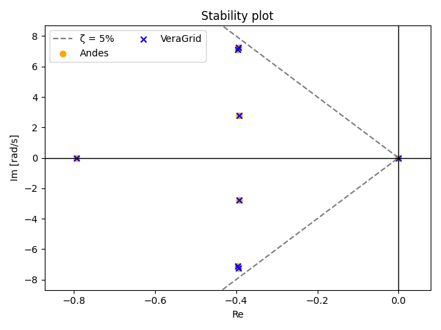
The following plot template is used to compare results.
import matplotlib.pyplot as plt
import numpy as np

x1 = VeraGrid_Eig.real
y1 = VeraGrid_Eig.imag
x2= Andes_Eig.real
y2 = Andes_Eig.imag
slope = 1 / 0.05
x_z = np.linspace(-200, 0, 400)
y_z = slope * x_z
# Plot the two lines (positive and negative imaginary axis)
plt.plot(x_z, y_z, '--', color='grey', label='$\lambda$ = 5%')
plt.plot(x_z, -y_z, '--', color='grey')
plt.scatter(x2, y2, marker='o', color='orange', label='Andes')
plt.scatter(x1, y1, marker='x', color='blue', label='VeraGrid')
plt.xlabel("Re [s -1]")
plt.ylabel("Im [s -1]")
plt.title("Stability plot")
margin_x = (x1.max() - x1.min()) * 0.1
margin_y = (y1.max() - y1.min()) * 0.1
x_min = x1.min() - margin_x
x_max = x1.max() + margin_x
y_min = y1.min() - margin_y
y_max = y1.max() + margin_y
plt.xlim([x_min, x_max])
plt.ylim([y_min, y_max])
plt.axhline(0, color='black', linewidth=1)  # eje horizontal (y = 0)
plt.axvline(0, color='black', linewidth=1)
plt.legend(loc='upper left', ncol=2)
plt.tight_layout()
plt.show()
Where VeraGrid_Eig and Andes_Eig are numpy arrays with the eigenvalues results from the VeraGrid and Andes
stability assessments respectively.
Small-signal
Small-signal analysis is a technique used to evaluate the dynamic behavior of nonlinear systems by linearizing their equations around a specific operating point. This approach assumes that perturbations are sufficiently small (typically within 1%) so that the system’s response can be approximated using linear models. The resulting linear representation enables the use of standard control engineering tools to assess system stability and dynamic performance.
Although small-signal analysis is inherently limited to small variations around the linearization point, it provides a robust framework for applying state-space models and a wide range of analytical techniques.
State-space representation
Small-signal stability assessment methods are typically classified into two main groups: state-space techniques and frequency-domain techniques. State-space methods model the system dynamics using a set of first-order differential equations


Where:
x : state variables vector
u : system inputs vector
y : outputs vector
A : state matrix
B : input matrix
C : output matrix
D : direct transmission matrix
This representation allows the representation of non-linear systems, time-dependent systems, autonomous systems and a wide range of possibilities. Moreover, each single system has infinite different state space models depending on how state variables and outputs are interpreted.
This formalism enables the representation of a wide variety of systems, including nonlinear, time-varying, and autonomous configurations. Importantly, a single physical system may admit infinitely many equivalent state-space realizations, depending on the choice of state variables and output definitions. This flexibility makes state-space modeling a powerful tool for both analysis and control design.
To perform a small-signal stability analysis, the system must first be linearized around a steady-state operating point. This process involves approximating the nonlinear system dynamics with a linear model that captures the system’s behavior under small perturbations.
In the context of state-space representation, linearization is achieved by expressing the system variables as deviations from their nominal operating points:


Substituting these into the original nonlinear model and applying a first-order Taylor expansion yields the linearized state-space representation:


Stability assessment
Eigenvalue analysis and participation factors (PFs) are key tools for identifying dominant modes and evaluating system stability. These methods are well established in conventional power systems and are increasingly being applied to power-electronics-based systems, where dynamic behavior is often more complex and sensitive to operating conditions.
The eigenvalues of the state matrix A (commonly referred to as the system’s modes) characterize its small-signal stability according to the following criteria:
All
 : asymptotically stable
All
 : marginally stable
At least one mode satisfies
: unstable
When a linearized system has complex conjugate modes, they represent oscillatory modes in the dynamic response.
The real part determines damping:
- : exponential decay
 : oscillations persist indefinitely
- : exponential growth
The imaginary part determines oscillation frequency:

In this line, Damping ratios are computed to assess oscillations on modes:
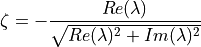
And they are analyzed as:
 : Unstable oscillations. The system exhibits exponentially growing modes due to eigenvalues with positive real part.
 : Marginally stable oscillations. The system sustains undamped oscillations indefinitely.
Eigenvalues lie on the imaginary axis.
: Marginally stable oscillations. The system sustains undamped oscillations indefinitely.
Eigenvalues lie on the imaginary axis. : Stable but oscillatory response. The system returns to equilibrium with decaying oscillations.
A commonly accepted threshold for adequate damping is around
: Stable but oscillatory response. The system returns to equilibrium with decaying oscillations.
A commonly accepted threshold for adequate damping is around  .
. : Critically damped response. The system returns to equilibrium without oscillations and in the shortest
possible time without overshoot.
: Critically damped response. The system returns to equilibrium without oscillations and in the shortest
possible time without overshoot.
Participation factors determine how much each state variable contributes to each mode and otherwise. In power systems it is crucial to determine which devices are the origin of the oscillations and instabilities. They are often normalized to to enhance interpretability and facilitate analytical comparison. They are computed as:

Where PF is the participation factor of the k-state variable to the i-mode, W is the left eigenvector of the k-state variable to the i-mode of matrix A and V is the right eigenvector of the k-state variable to the i-mode of matrix A.
DAE system to State Space representation
In power systems the dynamic behavior is described as a set of differential-algebraic equations (DAEs) due to the different components in the grid:
Differential equations arise with dynamic components such as synchronous generators, exciters, converters and control loops.
Algebraic equations come from network constraints and power balances mainly.
Explicit DAE formulation:


Merging the DAE formulation into the linearized state-space representation, the state matrix can be computed:

and therefore:

Where  ,
,  ,
,  and
and  are the
  ,
,  ,
,
 and
and  components of the jacobian matrix of
the DAE system respectively.
components of the jacobian matrix of
the DAE system respectively.
Benchmark - Kundur system
The Kundur two-area system is a standard benchmark network widely used for small-signal and transient stability studies. It was introduced in the P. Kundur power system stability literature as a compact, yet representative, test case that exposes inter-area oscillatory modes and control interactions without excessive model complexity.
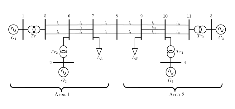
The main characteristics of the system, depicted in the figure above, are:
Two areas connected by a pair of parallel lines. In each area, 2 synchronous generators are placed so that each area can swing against each other and produce inter-area oscillations.
All the synchronous generators are connected to the network through a transformer.
In this version of the Kundur two-area system no shunts are connected to buses 7 and 9.
The base power is 100 MW and the voltage levels are 20kV for the generators and 230kV for the network.
The following code can be used to model the Kundur two area system without shunt in VeraGrid and to perform the small-signal Stability analysis.
from VeraGridEngine.Devices.multi_circuit import MultiCircuit
from VeraGridEngine.Devices.Substation.bus import Bus
from VeraGridEngine.Devices.Injections.generator import Generator
from VeraGridEngine.Devices.Injections.load import Load
from VeraGridEngine.Devices.Branches.line import Line

from VeraGridEngine.enumerations import DynamicIntegrationMethod, RmsInitializationMethod
from VeraGridEngine.Simulations.PowerFlow.power_flow_driver import PowerFlowOptions, PowerFlowDriver
from VeraGridEngine.Simulations.Rms.rms_options import RmsOptions
from VeraGridEngine.Simulations.SmallSignalStabilityRms.small_signal_driver import SmallSignalStabilityRmsDriver
from VeraGridEngine.Simulations.SmallSignalStabilityRms.small_signal_options import (
    RmsSmallSignalStabilityOptions,
)
import VeraGridEngine.api as gce

grid = MultiCircuit()

# Buses
bus1 = Bus(name="Bus1", Vnom=230)
bus2 = Bus(name="Bus2", Vnom=230)
bus3 = Bus(name="Bus3", Vnom=230, is_slack=True)
bus4 = Bus(name="Bus4", Vnom=230)
bus5 = Bus(name="Bus5", Vnom=230)
bus6 = Bus(name="Bus6", Vnom=230)
bus7 = Bus(name="Bus7", Vnom=230)
bus8 = Bus(name="Bus8", Vnom=230)
bus9 = Bus(name="Bus9", Vnom=230)
bus10 = Bus(name="Bus10", Vnom=230)
bus11 = Bus(name="Bus11", Vnom=230)

grid.add_bus(bus1)
grid.add_bus(bus2)
grid.add_bus(bus3)
grid.add_bus(bus4)
grid.add_bus(bus5)
grid.add_bus(bus6)
grid.add_bus(bus7)
grid.add_bus(bus8)
grid.add_bus(bus9)
grid.add_bus(bus10)
grid.add_bus(bus11)

# Line
line0 = grid.add_line(
    Line(name="line 5-6-1", bus_from=bus5, bus_to=bus6,
         r=0.00500, x=0.05000, b=0.02187, rate=750.0))

line1 = grid.add_line(
    Line(name="line 5-6-2", bus_from=bus5, bus_to=bus6,
         r=0.00500, x=0.05000, b=0.02187, rate=750.0))

line2 = grid.add_line(
    Line(name="line 6-7-1", bus_from=bus6, bus_to=bus7,
         r=0.00300, x=0.03000, b=0.00583, rate=700.0))

line3 = grid.add_line(
    Line(name="line 6-7-2", bus_from=bus6, bus_to=bus7,
         r=0.00300, x=0.03000, b=0.00583, rate=700.0))

line4 = grid.add_line(
    Line(name="line 6-7-3", bus_from=bus6, bus_to=bus7,
         r=0.00300, x=0.03000, b=0.00583, rate=700.0))

line5 = grid.add_line(
    Line(name="line 7-8-1", bus_from=bus7, bus_to=bus8,
         r=0.01100, x=0.11000, b=0.19250, rate=400.0))

line6 = grid.add_line(
    Line(name="line 7-8-2", bus_from=bus7, bus_to=bus8,
         r=0.01100, x=0.11000, b=0.19250, rate=400.0))

line7 = grid.add_line(
    Line(name="line 8-9-1", bus_from=bus8, bus_to=bus9,
         r=0.01100, x=0.11000, b=0.19250, rate=400.0))

line8 = grid.add_line(
    Line(name="line 8-9-2", bus_from=bus8, bus_to=bus9,
         r=0.01100, x=0.11000, b=0.19250, rate=400.0))

line9 = grid.add_line(
    Line(name="line 9-10-1", bus_from=bus9, bus_to=bus10,
         r=0.00300, x=0.03000, b=0.00583, rate=700.0))

line10 = grid.add_line(
    Line(name="line 9-10-2", bus_from=bus9, bus_to=bus10,
         r=0.00300, x=0.03000, b=0.00583, rate=700.0))

line11 = grid.add_line(
    Line(name="line 9-10-3", bus_from=bus9, bus_to=bus10,
         r=0.00300, x=0.03000, b=0.00583, rate=700.0))

line12 = grid.add_line(
    Line(name="line 10-11-1", bus_from=bus10, bus_to=bus11,
         r=0.00500, x=0.05000, b=0.02187, rate=750.0))

line13 = grid.add_line(
    Line(name="line 10-11-2", bus_from=bus10, bus_to=bus11,
         r=0.00500, x=0.05000, b=0.02187, rate=750.0))

# Transformers
grid.add_line(
    Line(name="trafo 5-1", bus_from=bus5, bus_to=bus1,
         r=0.00000, x=0.15 * (100.0 / 900.0), b=0.0, rate=900.0))

grid.add_line(
    Line(name="trafo 6-2", bus_from=bus6, bus_to=bus2,
         r=0.00000, x=0.15 * (100.0 / 900.0), b=0.0, rate=900.0))

grid.add_line(
    Line(name="trafo 11-3", bus_from=bus11, bus_to=bus3,
         r=0.00000, x=0.15 * (100.0 / 900.0), b=0.0, rate=900.0))

grid.add_line(
    Line(name="trafo 10-4", bus_from=bus10, bus_to=bus4,
         r=0.00000, x=0.15 * (100.0 / 900.0), b=0.0, rate=900.0))

# load
load1 = Load(name="load1", P=967.0, Q=100.0, Pl0=-9.670000000007317, Ql0=-0.9999999999967969)
grid.add_load(bus=bus7, api_obj=load1)

load2 = Load(name="load2", P=1767.0, Q=100.0, Pl0=-17.6699999999199, Ql0=-0.999999999989467)
grid.add_load(bus=bus9, api_obj=load2)

# Generators
fn_1 = 60.0
M_1 = 13.0 * 9.0
D_1 = 10.0 * 9.0
ra_1 = 0.0
xd_1 = 0.3 * 100.0 / 900.0
omega_ref_1 = 1.0
Kp_1 = 0.0
Ki_1 = 0.0

fn_2 = 60.0
M_2 = 13.0 * 9.0
D_2 = 10.0 * 9.0
ra_2 = 0.0
xd_2 = 0.3 * 100.0 / 900.0
omega_ref_2 = 1.0
Kp_2 = 0.0
Ki_2 = 0.0

fn_3 = 60.0
M_3 = 12.35 * 9.0
D_3 = 10.0 * 9.0
ra_3 = 0.0
xd_3 = 0.3 * 100.0 / 900.0
omega_ref_3 = 1.0
Kp_3 = 0.0
Ki_3 = 0.0

fn_4 = 60.0
M_4 = 12.35 * 9.0
D_4 = 10.0 * 9.0
ra_4 = 0.0
xd_4 = 0.3 * 100.0 / 900.0
omega_ref_4 = 1.0
Kp_4 = 0.0
Ki_4 = 0.0

# Generators
gen1 = Generator(
    name="Gen1", P=700.0, vset=1.03, Snom=900.0,
    x1=xd_1, r1=ra_1, freq=fn_1,
    tm0=6.999999999999923,
    vf=1.141048034212655,
    M=M_1, D=D_1,
    omega_ref=omega_ref_1,
    Kp=Kp_1, Ki=Ki_1
)

gen2 = Generator(
    name="Gen2", P=700.0, vset=1.01, Snom=900.0,
    x1=xd_2, r1=ra_2, freq=fn_2,
    tm0=6.999999999999478,
    vf=1.180101792122771,
    M=M_2, D=D_2,
    omega_ref=omega_ref_2,
    Kp=Kp_2, Ki=Ki_2
)

gen3 = Generator(
    name="Gen3", P=719.091, vset=1.03, Snom=900.0,
    x1=xd_3, r1=ra_3, freq=fn_3,
    tm0=7.331832804674334,
    vf=1.1551307366822237,
    M=M_3, D=D_3,
    omega_ref=omega_ref_3,
    Kp=Kp_3, Ki=Ki_3
)

gen4 = Generator(
    name="Gen4", P=700.0, vset=1.01, Snom=900.0,
    x1=xd_4, r1=ra_4, freq=fn_4,
    tm0=6.99999999999765,
    vf=1.2028205849036708,
    M=M_4, D=D_4,
    omega_ref=omega_ref_4,
    Kp=Kp_4, Ki=Ki_4
)

grid.add_generator(bus=bus1, api_obj=gen1)
grid.add_generator(bus=bus2, api_obj=gen2)
grid.add_generator(bus=bus3, api_obj=gen3)
grid.add_generator(bus=bus4, api_obj=gen4)

# # Run power flow
pf_options = PowerFlowOptions(
    solver_type=gce.SolverType.NR,
    retry_with_other_methods=False,
    verbose=0,
    initialize_with_existing_solution=True,
    tolerance=1e-8,
    max_iter=25,
    control_q=False,
    control_taps_modules=True,
    control_taps_phase=True,
    control_remote_voltage=True,
    orthogonalize_controls=True,
    apply_temperature_correction=True,
    branch_impedance_tolerance_mode=gce.BranchImpedanceMode.Specified,
    distributed_slack=False,
    ignore_single_node_islands=False,
    trust_radius=1.0,
    backtracking_parameter=0.05,
    use_stored_guess=False,
    initialize_angles=False,
    generate_report=False,
    three_phase_unbalanced=False
)
power_flow = PowerFlowDriver(grid, pf_options)
power_flow.run()
res = power_flow.results

# # Print results
print(res.get_bus_df())
print(res.get_branch_df())
print(f"Converged: {res.converged}")

# Small-signal stability assessment at t = 0 s.
rms_options = RmsOptions(
    time_step=0.001,
    simulation_time=10.0,
    tolerance=1e-6,
    integration_method=DynamicIntegrationMethod.DaeBackEuler,
    initialization_method=RmsInitializationMethod.Explicit,
    use_init_values=False,
    max_iter=1000,
    verbose=0,
)

ss_options = RmsSmallSignalStabilityOptions(
    ss_assessment_time=0.0,
    k=0,
    verbose=1,
)

small_signal_driver = SmallSignalStabilityRmsDriver(
    grid=grid,
    rms_options=rms_options,
    sss_options=ss_options,
    pf_results=res,
)
small_signal_driver.run()

Eigenvalues = small_signal_driver.results.eigenvalues
PFactors = small_signal_driver.results.participation_factors
damping_ratios = small_signal_driver.results.damping_ratios
conjugate_frequencies = small_signal_driver.results.conjugate_frequencies
state_matrix = small_signal_driver.results.state_matrix

plot_stability(Eigenvalues, plot_units="rad/s")