from trunk.ai.ai_iterable_example import grid_

💥 Contingency analysis

VeraGrid has contingency simulations, and it features a quite flexible way of defining contingencies. First you define a contingency group, and then define individual events that are assigned to that contingency group. The simulation then tries all the contingency groups and apply the events registered in each group.

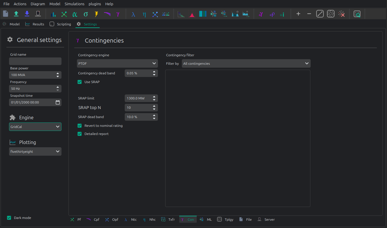
• Contingency method or engine:

  • “Power flow”: Base flows are obtained with a power flow according to pf_options. Each contingency is obtained by runnig a power flow also according to pf_options and to the more sophisticated contingency definition.

  • “Linear”: Base flows are taken from options.Pf or if not provided, computed linearly. The continegencies are computed linearly, according to the more sophisticated contingency definition.

  • “PTDF Scan”: Brute contingency scan, this is the fastest and may not adhere to the sophisticated contingency definition. No SRAP or particular condition is performed.

Registered Result Properties

ContingencyAnalysisResults registered properties

The snapshot contingency analysis result stores the post-contingency network quantities and report object.

Property	Type	Description
branch_names	StrVec	Names aligned with branch-indexed result arrays.
bus_names	StrVec	Names aligned with bus-indexed result arrays.
con_names	StrVec	Names aligned with contingency-indexed result arrays.
bus_types	IntVec	Bus type code used by the solved numerical model.
voltage	CxMat	Complex bus voltage solution.
Sbus	CxMat	Complex bus power injection.
Sf	CxMat	Complex branch power flow at the from side.
loading	CxMat	Branch loading result.
srap_used_power	Mat	SRAP remedial action power used in the contingency study.
report	ContingencyResultsReport	Detailed report object produced by the study.

ContingencyAnalysisTimeSeriesResults registered properties

The time-series contingency analysis result stores aggregate contingency limits and overload statistics per time step.

Property	Type	Description
branch_names	StrVec	Names aligned with branch-indexed result arrays.
bus_names	StrVec	Names aligned with bus-indexed result arrays.
bus_types	IntVec	Bus type code used by the solved numerical model.
con_names	StrVec	Names aligned with contingency-indexed result arrays.
S	Mat	Complex bus power result matrix.
max_flows	Mat	Maximum branch flow observed across contingencies.
max_loading	Mat	Maximum branch loading observed across contingencies.
sum_overload	Mat	Sum of overload values across contingencies.
mean_overload	Mat	Mean overload value across contingencies.
std_dev_overload	Mat	Standard deviation of overload values across contingencies.
srap_used_power	Mat	SRAP remedial action power used in the contingency study.
report	ContingencyResultsReport	Detailed report object produced by the study.

API

Snapshot contingency analysis

import os
import VeraGridEngine as gce

folder = os.path.join('Grids_and_profiles', 'grids')
fname = os.path.join(folder, 'IEEE 5 Bus.xlsx')

grid = gce.open_file(fname)

branches = grid.get_branches()

# manually generate the contingencies
for i, br in enumerate(branches):
  # add a contingency group
  group = gce.ContingencyGroup(name="contingency {}".format(i + 1))
  grid.add_contingency_group(group)

  # add the branch contingency to the groups, only groups are failed at once
  con = gce.Contingency(device=br, name=br.name, group=group)
  grid.add_contingency(con)

# add a special contingency
group = gce.ContingencyGroup(name="Special contingency")
grid.add_contingency_group(group)
grid.add_contingency(gce.Contingency(device=branches[3], name=branches[3].name, group=group))
grid.add_contingency(gce.Contingency(device=branches[5], name=branches[5].name, group=group))

pf_options = gce.PowerFlowOptions(solver_type=gce.SolverType.NR)

# declare the contingency options
options_ = gce.ContingencyAnalysisOptions(
    
  # Contingency method to use
  contingency_method=gce.ContingencyMethod.PowerFlow,

  # optional, you can send here any contingency groups
  contingency_groups=grid.get_contingency_groups(),
  
  # if no power flow options are provided
  # a linear power flow is used
  pf_options=pf_options
)

# Get all the defined contingency groups from the circuit
contingency_groups = grid.get_contingency_groups()

# Pass the list of contingency groups as required (optional)
linear_multiple_contingencies = gce.LinearMultiContingencies(grid=grid,
                                                             contingency_groups_used=contingency_groups)

simulation = gce.ContingencyAnalysisDriver(grid=grid,
                                           options=options_,
                                           linear_multiple_contingencies=linear_multiple_contingencies)

simulation.run()

# print results
df = simulation.results.mdl(gce.ResultTypes.BranchActivePowerFrom).to_df()
print("Contingency flows:\n", df)

Output:

Contingency flows:
                       Branch 0-1  Branch 0-3  Branch 0-4  Branch 1-2  Branch 2-3  Branch 3-4
# contingency 1          0.000000  322.256814 -112.256814 -300.000000 -277.616985 -350.438026
# contingency 2        314.174885    0.000000 -104.174887   11.387545   34.758624 -358.359122
# contingency 3        180.382705   29.617295    0.000000 -120.547317  -97.293581 -460.040537
# contingency 4        303.046401  157.540574 -250.586975    0.000000   23.490000 -214.130663
# contingency 5        278.818887  170.710914 -239.529801  -23.378976    0.000000 -225.076976
# contingency 6        323.104522  352.002620 -465.107139   20.157096   43.521763    0.000000
# Special contingency  303.046401  372.060738 -465.107139    0.000000   23.490000    0.000000

This simulation can also be done for time series.

Contingency analysis time series

To perform the contingency analysis of a time series, it’s easier to directly usi the API:

import os
import VeraGridEngine as gce

folder = os.path.join('Grids_and_profiles', 'grids')
fname = os.path.join(folder, 'IEEE39_1W.veragrid')
main_circuit = gce.open_file(fname)

results = gce.contingencies_ts(circuit=main_circuit,
                               detailed_massive_report=False,
                               contingency_deadband=0.0,
                               contingency_method=gce.ContingencyMethod.PowerFlow)

Note that the grid must have the declared contingencies saved already. Also note that the results are statistics, and you will not get a cube because for large grids that demands terabytes of RAM memory.