🌀 State estimation

State estimation in VeraGrid reconstructs the electrical state of the network from measurements instead of assuming that all bus injections and branch conditions are perfectly known.

Its objective is to infer the most likely bus voltages, angles, flows, and injections that best fit the available measurements.

This is the standard study to use when the network model is known but the real-time operating point is only partially observed through telemetry.

What The Study Evaluates

The state estimation study combines:

• the network model

• the available measurements

• the measurement uncertainty

to estimate:

• bus voltage magnitudes

• bus voltage angles

• bus active and reactive injections

• branch active and reactive flows

• branch currents, loading, and losses

Unlike a standard power flow, the operating point is not prescribed directly from deterministic injections. Instead, it is inferred from the measurement set.

Supported Measurements

The driver collects measurements already attached to the network model.

The current implementation supports:

• bus active power injection measurements

• bus reactive power injection measurements

• generator active power measurements

• generator reactive power measurements

• bus voltage magnitude measurements

• bus voltage angle measurements

• branch active power flow measurements on the from side

• branch active power flow measurements on the to side

• branch reactive power flow measurements on the from side

• branch reactive power flow measurements on the to side

• branch current magnitude measurements on the from side

• branch current magnitude measurements on the to side

Each measurement carries both:

• a measured value

• a standard deviation or uncertainty

That uncertainty is essential because the estimator weighs measurements according to their confidence.

Observability

A state estimator can only recover the network state if the measurement set is sufficiently informative.

This is the observability problem:

• if the system is observable, the estimator has enough information to solve for the state

• if the system is not observable, some buses or variables cannot be uniquely inferred from the available measurements

VeraGrid can run an observability analysis before solving the estimator. When enabled, the driver can:

• detect unobservable buses

• profile the contribution of measurements

• optionally add pseudo-measurements for unobservable buses

This is especially useful when building new telemetry sets or validating whether a measurement configuration is sufficient for state estimation.

Pseudo-Measurements

If the network is not fully observable, VeraGrid can augment the measurement set with pseudo-measurements.

Pseudo-measurements are synthetic measurements, usually with a relatively high uncertainty, that help make the system observable enough to solve.

They are useful when:

• some buses have no direct telemetry

• the measurement set is incomplete

• a practical solution is preferred over rejecting the case as unobservable

The driver records the pseudo-measurements it injects so they can be inspected later through the convergence reports.

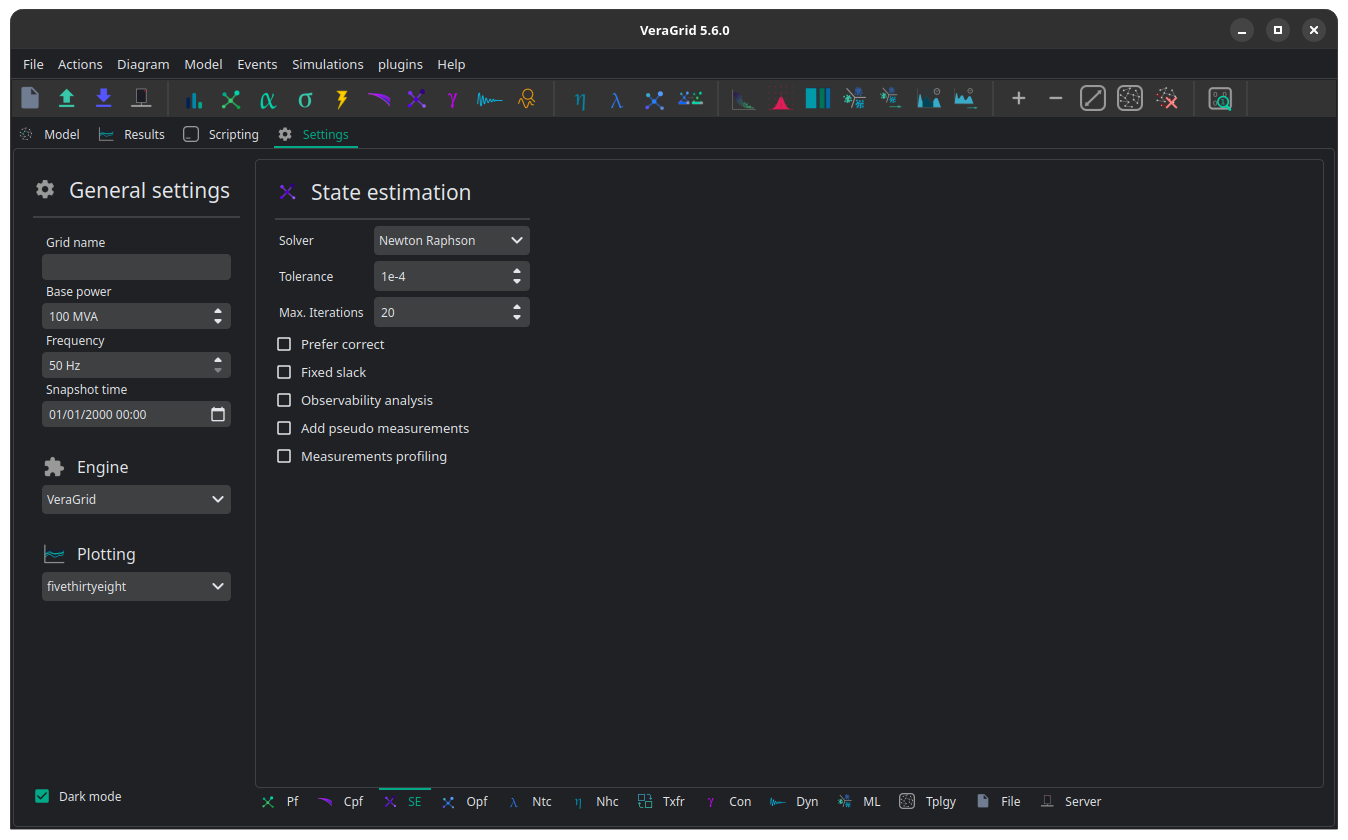
Solvers

The state estimation driver currently supports several numerical solvers through StateEstimationOptions:

• SolverType.NR: Newton-Raphson

• SolverType.LM: Levenberg-Marquardt

• SolverType.GN: Gauss-Newton

• SolverType.Decoupled_LU: decoupled state estimation

In general:

• use Newton-Raphson as the default robust choice

• use Levenberg-Marquardt when a damped method is preferred

• use Gauss-Newton for the classical least-squares style formulation

• use Decoupled when a faster approximate approach is acceptable

Main Options

The main state estimation options are:

• solver: numerical method used to solve the estimator

• tol: convergence tolerance

• max_iter: maximum number of iterations

• verbose: solver verbosity

• prefer_correct: whether correction is preferred over measurement deletion in bad-data handling logic

• c_threshold: confidence threshold used in bad-data related logic

• fixed_slack: whether slack-bus measurements are omitted from the formulation

• run_observability_analyis: enables observability analysis before estimation

• add_pseudo_measurements: injects pseudo-measurements when unobservable buses are detected

• run_measurement_profiling: enables measurement contribution profiling

• include_line_measurements_on_both_ends: controls how line-end measurements are considered during observability analysis

• pseudo_meas_std: standard deviation assigned to created pseudo-measurements

Result Object

The study returns a StateEstimationResults object.

It exposes the estimated electrical state through arrays and convenience methods.

Main result arrays include:

• voltage

• Sbus

• Sf, St

• If, It

• loading

• losses

Convenience methods include:

• get_bus_df()

• get_branch_df()

• get_report_dataframe(island_idx=0)

The result object also stores convergence_reports, one per island, which contain:

• convergence status

• error

• elapsed time

• iteration count

• bad-data detection status

• observability status

• unobservable buses

• pseudo-measurements

• measurement profiling information

Interpretation Notes

• A converged solution does not automatically mean the measurement set was good; always inspect observability and bad-data information as well.

• If pseudo-measurements were needed, the estimate is usable but less grounded in direct telemetry.

• If the network splits into islands, each island is solved separately and has its own convergence report.

• The quality of the estimate depends strongly on both the placement and the uncertainty values of the measurements.

Registered Result Properties

StateEstimationResults registered properties

The state-estimation result stores estimated network quantities and bad-data status.

Property	Type	Description
bus_names	StrVec	Names aligned with bus-indexed result arrays.
branch_names	StrVec	Names aligned with branch-indexed result arrays.
hvdc_names	StrVec	Names aligned with HVDC line-indexed result arrays.
gen_names	StrVec	Names aligned with generator-indexed result arrays.
batt_names	StrVec	Names aligned with battery-indexed result arrays.
sh_names	StrVec	Names aligned with shunt-indexed result arrays.
bus_types	IntVec	Bus type code used by the solved numerical model.
F	IntVec	Branch from-bus index for each branch.
T	IntVec	Branch to-bus index for each branch.
hvdc_F	IntVec	HVDC from-bus index for each HVDC line.
hvdc_T	IntVec	HVDC to-bus index for each HVDC line.
bus_area_indices	IntVec	Area index assigned to each bus.
area_names	IntVec	Area names or area identifiers used for inter-area aggregation.
Sbus	CxVec	Complex bus power injection.
voltage	CxVec	Complex bus voltage solution.
Sf	CxVec	Complex branch power flow at the from side.
St	CxVec	Complex branch power flow at the to side.
If	CxVec	Complex branch current at the from side.
It	CxVec	Complex branch current at the to side.
tap_module	Vec	Transformer tap module used in the solved state.
tap_angle	Vec	Transformer tap angle used in the solved state.
Vbranch	CxVec	Complex branch voltage result used by branch reports.
loading	CxVec	Branch loading result.
losses	CxVec	Complex branch losses.
losses_hvdc	Vec	Losses result.
Pf_hvdc	Vec	Registered result field Pf_hvdc.
Pt_hvdc	Vec	Registered result field Pt_hvdc.
loading_hvdc	Vec	Loading result.
losses_vsc	Vec	Losses result.
Pf_vsc	Vec	VSC result field Pf_vsc.
St_vsc	CxVec	Complex branch power flow at the to side.
If_vsc	Vec	Complex branch current at the from side.
It_vsc	CxVec	Complex branch current at the to side.
loading_vsc	Vec	Loading result.
gen_q	Vec	Generator reactive power output.
battery_q	Vec	Battery reactive power output.
shunt_q	Vec	Shunt reactive power output.
bad_data_detected	bool	Flag indicating whether bad data was detected by the estimator.

API

The following example is based on the classic three-bus reference from A. Monticelli’s book.

import VeraGridEngine as gce

m_circuit = gce.MultiCircuit()

b1 = gce.Bus('B1', is_slack=True)
b2 = gce.Bus('B2')
b3 = gce.Bus('B3')

br1 = gce.Line(b1, b2, name='Br1', r=0.01, x=0.03, rate=100.0)
br2 = gce.Line(b1, b3, name='Br2', r=0.02, x=0.05, rate=100.0)
br3 = gce.Line(b2, b3, name='Br3', r=0.03, x=0.08, rate=100.0)

# add measurements
m_circuit.add_pf_measurement(gce.PfMeasurement(0.888, 0.008, br1))
m_circuit.add_pf_measurement(gce.PfMeasurement(1.173, 0.008, br2))

m_circuit.add_qf_measurement(gce.QfMeasurement(0.568, 0.008, br1))
m_circuit.add_qf_measurement(gce.QfMeasurement(0.663, 0.008, br2))

m_circuit.add_pi_measurement(gce.PiMeasurement(-0.501, 0.01, b2))
m_circuit.add_qi_measurement(gce.QiMeasurement(-0.286, 0.01, b2))

m_circuit.add_vm_measurement(gce.VmMeasurement(1.006, 0.004, b1))
m_circuit.add_vm_measurement(gce.VmMeasurement(0.968, 0.004, b2))

m_circuit.add_bus(b1)
m_circuit.add_bus(b2)
m_circuit.add_bus(b3)

m_circuit.add_line(br1)
m_circuit.add_line(br2)
m_circuit.add_line(br3)

se = gce.StateEstimationDriver(circuit=m_circuit)
se.run()

print(se.results.get_bus_df())
print(se.results.get_branch_df())

Output:

          Vm        Va         P        Q
B1  0.999629  0.000000  2.064016  1.22644
B2  0.974156 -1.247547  0.000000  0.00000
B3  0.943890 -2.745717  0.000000  0.00000

            Pf        Qf          Pt         Qt    loading    Ploss    Qloss
Br1  89.299199 55.882169  -88.188659 -52.550550  89.299199 1.110540 3.331619
Br2 117.102446 66.761871 -113.465724 -57.670065 117.102446 3.636722 9.091805
Br3  38.591163 22.775597  -37.956374 -21.082828  38.591163 0.634789 1.692770

Using explicit options:

import VeraGridEngine as gce

options = gce.StateEstimationOptions(
    solver=gce.SolverType.NR,
    tol=1e-8,
    max_iter=100,
    run_observability_analyis=True,
    add_pseudo_measurements=True,
    run_measurement_profiling=True,
    pseudo_meas_std=1.0,
)

drv = gce.StateEstimationDriver(circuit=m_circuit, options=options)
drv.run()

print("Converged:", drv.results.converged)
print("Error:", drv.results.error)
print(drv.results.get_report_dataframe())

Inspecting the convergence and observability report:

report = drv.results.convergence_reports[0]

print("Bad data detected:", report.get_bad_data_detected())
print("Unobservable buses:", report.get_unobservable_buses())
print("Pseudo measurements:", report.get_pseudo_measurements())
print("Measurement profile:", report.get_measurement_profile())

Accessing result tables:

from VeraGridEngine.enumerations import ResultTypes

bus_vm_table = drv.results.mdl(ResultTypes.BusVoltageModule)
branch_loading_table = drv.results.mdl(ResultTypes.BranchLoading)

print(bus_vm_table.data)
print(branch_loading_table.data)

Practical Guidance

• Start by checking observability before tuning solver settings.

• Use realistic measurement standard deviations; arbitrary values can distort the estimator strongly.

• Prefer adding a few well-placed real measurements over relying heavily on pseudo-measurements.

• Inspect get_report_dataframe() and convergence_reports, not only the estimated voltages and flows.

• If the estimate looks strange, verify both the measurement values and the device associations first.