➿ Continuation power flow

VeraGrid can run continuation power flows (voltage collapse studies)

Max. Iterations Number of iteration to perform at each voltage stability (predictor-corrector) stage.

Stop at Point of the curve to top at

- Nose: Stop at the voltage collapse point
- Full: Trace the full curve.

Use alpha target from the base situation The voltage collapse (stability) simulation is a “travel” from a base situation towards a “final” one. When this mode is selected the final situation is a linear combination of the base situation. All the power values are multiplied by the same number.

Use departure and target points from time series When this option is selected the base and the target points are given by time series points. This allows that the base and the final situations to have non even relationships while evolving from the base situation to the target situation.

Registered Result Properties

ContinuationPowerFlowResults registered properties

The continuation power flow result stores the solved continuation path and branch quantities at each continuation step.

Property	Type	Description
bus_names	StrVec	Names aligned with bus-indexed result arrays.
branch_names	StrVec	Names aligned with branch-indexed result arrays.
bus_types	IntVec	Bus type code used by the solved numerical model.
voltages	CxMat	Complex bus voltage solutions along the continuation path.
lambdas	Vec	Continuation loading parameter values.
error	Vec	Solver error or residual value.
converged	BoolVec	Convergence flag for the solved case or time step.
Sf	CxMat	Complex branch power flow at the from side.
St	CxMat	Complex branch power flow at the to side.
loading	CxMat	Branch loading result.
losses	CxMat	Complex branch losses.
Sbus	CxMat	Complex bus power injection.

SigmaAnalysisResults registered properties

The sigma analysis result stores the sigma-plane values and distances used by the voltage-stability assessment.

Property	Type	Description
lambda_value	float	Loading parameter used by the sigma analysis.
bus_names	StrVec	Names aligned with bus-indexed result arrays.
Sbus	CxVec	Complex bus power injection.
distances	Vec	Distance of each bus point to the sigma stability boundary.
sigma_re	Vec	Real component of the sigma-plane value.
sigma_im	Vec	Imaginary component of the sigma-plane value.

API

Snapshot continuation power flow

import os
from matplotlib import pyplot as plt
import VeraGridEngine as gce

plt.style.use('fivethirtyeight')

folder = os.path.join('..', 'Grids_and_profiles', 'grids')
fname = os.path.join(folder, 'South Island of New Zealand.veragrid')

# open the grid file
main_circuit = gce.open_file(fname)

# Run the continuation power flow with the default options
# Since we do not provide any power flow results, it will run one for us
results = gce.continuation_power_flow(grid=main_circuit,
                                      factor=2.0,
                                      stop_at=gce.CpfStopAt.Full)

# plot the results
fig = plt.figure(figsize=(18, 6))

ax1 = fig.add_subplot(121)
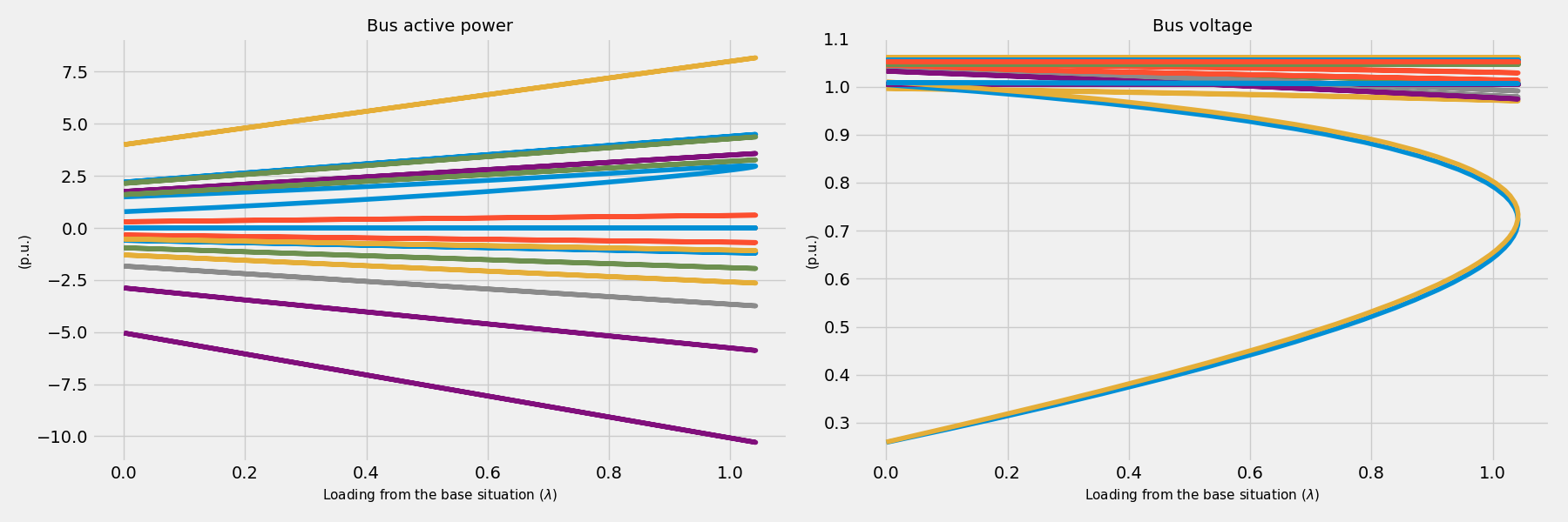
res = results.mdl(gce.ResultTypes.BusActivePower)
res.plot(ax=ax1)

ax2 = fig.add_subplot(122)
res = results.mdl(gce.ResultTypes.BusVoltageModule)
res.plot(ax=ax2)

plt.tight_layout()

plt.show()

A more elaborated way to run the simulation, controlling all the steps:

import os
from matplotlib import pyplot as plt
import VeraGridEngine as gce

plt.style.use('fivethirtyeight')

folder = os.path.join('..', 'Grids_and_profiles', 'grids')
fname = os.path.join(folder, 'South Island of New Zealand.veragrid')

# open the grid file
main_circuit = gce.FileOpen(fname).open()

# we need to initialize with a power flow solution
pf_options = gce.PowerFlowOptions()
power_flow = gce.PowerFlowDriver(grid=main_circuit, options=pf_options)
power_flow.run()

# declare the CPF options
vc_options = gce.ContinuationPowerFlowOptions(step=0.001,
                                              approximation_order=gce.CpfParametrization.ArcLength,
                                              adapt_step=True,
                                              step_min=0.00001,
                                              step_max=0.2,
                                              error_tol=1e-3,
                                              tol=1e-6,
                                              max_it=20,
                                              stop_at=gce.CpfStopAt.Full,
                                              verbose=False)

# We compose the target direction
factor = 2.0
base_power = power_flow.results.Sbus / main_circuit.Sbase
vc_inputs = gce.ContinuationPowerFlowInput(Sbase=base_power,
                                           Vbase=power_flow.results.voltage,
                                           Starget=base_power * factor)

# declare the CPF driver and run
vc = gce.ContinuationPowerFlowDriver(grid=main_circuit,
                                     options=vc_options,
                                     inputs=vc_inputs,
                                     pf_options=pf_options)
vc.run()

# plot the results
fig = plt.figure(figsize=(18, 6))

ax1 = fig.add_subplot(121)
res = vc.results.mdl(gce.ResultTypes.BusActivePower)
res.plot(ax=ax1)

ax2 = fig.add_subplot(122)
res = vc.results.mdl(gce.ResultTypes.BusVoltageModule)
res.plot(ax=ax2)

plt.tight_layout()

plt.show()

Theory

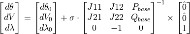
The continuation power flow is a technique that traces a trajectory from a base situation given to a combination of power and voltage , to another situation determined by another combination of power . When the final power situation is undefined, then the algorithm continues until the Jacobian is singular, tracing the voltage collapse curve.

The method uses a predictor-corrector technique to trace this trajectory.

Predictor step

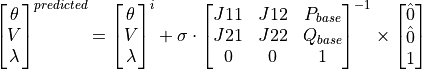
Corrector step